Estimating the Margin of Gait Stability in Healthy Elderly Using the Triaxial Kinematic Motion of a Single Body Feature

Abstract

Gait stability indices are crucial for identifying individuals at risk of falling while walking. The margin of stability is one such index, known for its good construct validity. Generally, the measurement of this stability index requires a motion capture system, rendering it inaccessible for everyday use. This study proposes an alternative approach by estimating the index through time-series data of triaxial kinematic motion from a single body feature. We analyzed an open gait database comprising data from 60 participants aged over 60 to identify the most accurate body feature for estimating the margin of stability. The margin of stability values were estimated by using principal motion analysis, with the time series of the triaxial translational velocities of a body feature as predictors. Among the 10 body feature points, the sacral crest provided the highest accuracy, with the correlation coefficients between observation and estimation being 0.56 and 0.54 for the mediolateral and anterior directions, respectively. Although these values need to be further improved, these findings pave the way for developing an accessible system to estimate fall risks.

1. Introduction

A variety of gait stability indices have been investigated to identify individuals at a high risk of falling [1,2]. A common objective of these indices is to facilitate the identification of such individuals, enabling the provision of appropriate interventions to mitigate fall risks [3]. In the pursuit of accessible measures for assessing fall risks, the potential of inertial measurement units (IMUs) for gait analysis has garnered significant interest [4,5,6,7,8,9,10]. For instance, Kim et al. [4] employed an IMU sensor embedded in a shoe to calculate basic gait parameters such as stride and walking speed. Jebelli et al. [6] distinguished between the maximum Lyapunov exponents of cyclic gait patterns, measured by using IMU sensors attached to the lower thigh, in individuals bearing different loads. Yang et al. [9] developed a prototype of a real-time warning system for falls using an IMU sensor placed inside a jacket.

The margin of stability (MoS) [11,12] is a gait stability index recognized for its strong construct validity. As outlined in Section 2.2, it is derived from the kinematic stability of an inverted pendulum model, representing a simplified walking figure. This index is instrumental in assessing the risk of falling due to postural instability during both normal and perturbed walking in healthy individuals as well as those with pathological gait conditions [13]. Although the MoS can be defined for all directions [14], it is commonly calculated for the anterior and mediolateral directions. Thus far, numerous studies have focused on the MoS [15,16,17,18,19,20,21,22]. For instance, Ohtsu et al. [15] explored various representative values of the MoS, such as mean and integral values, during a gait cycle among healthy young adults to establish a reference base. Harro et al. [16] found that individuals with Parkinson’s disease exhibited higher MoS values than a healthy control group, indicating a difference in walking strategy between groups at high and low fall risks. Such a conservative strategy has typically been observed in the elderly [17,23,24]. Additionally, the response of postural stability to unexpected treadmill movements has been analyzed using the MoS [19,22]. Sivakumaran et al. [25] linked the variability of gait parameters with MoS variability, proposing that individuals adjust spatiotemporal gait patterns to preserve postural stability. Thus, the MoS serves as a reliable indicator of postural stability during walking under various conditions.

The computation of the MoS necessitates the simultaneous measurement of multiple body points, typically requiring an optical or IMU-based [10] motion capture system, limiting MoS recordings to laboratory settings. However, if the MoS is estimated, using devices such as IMUs embedded in smartphones, this can increase awareness among people about their gait instability and falling risk. Although the computation of the MoS demands positions from multiple body points, the synergy in human motion suggests that measuring fewer points might suffice for estimating the MoS. Iwasaki et al. [26] estimated the mediolateral MoS from the triaxial velocities of the center of body mass in healthy elderly participants, achieving a correlation coefficient of 0.55 between the observed and estimated values. The estimation accuracy can potentially be enhanced by including the angular velocities of body segments [27]. While these studies [26,27] affirm the feasibility of estimating the MoS using a single IMU, the question of estimate accuracy persists. This concern arises because accurately computing the MoS requires kinematic information from at least three body features: the center of body mass and both feet [11,12]. Therefore, this study identified conditions that can improve the estimation accuracy, specifically determining the most suitable body points for predicting the MoS.

We compared 10 body feature points in terms of the accuracy of the anterior and mediolateral MoSs. To this end, a principal motion analysis (PMA) [26,28] has been conducted using triaxial translational velocities. This study builds upon our previous study [29], which compared three body points, including seven additional feature points, using nuanced statistical methods, specifically cross-validation. While the sacral crest was identified as one of the most promising feature points in our earlier work [29], this study explores the potential of discovering other suitable points. Although this study relies on data recorded by an optical motion capture system, identifying suitable body points advances us toward accessible MoS measurements using an IMU.

2. Materials and Methods

2.1. Data Used for Analysis

We employed an open database from the National Institute of Advanced Industrial Science and Technology [30], where the motion data of gait are recorded for 300 healthy Japanese individuals with the ethical approval of the local review committee. Thus far, the same database has been employed in many studies, e.g., [17,31,32,33]. For our analysis, we selected data from 60 individuals, comprising 30 males and 30 females randomly chosen, all above the age of 60 years. The means and standard deviations of their height and weight were 159.62 ± 7.58 cm and 60.57 ± 9.33 kg, respectively. They walked in a 10 m straight line in bare feet with a mean (±standard deviation) stride length and step width of 1.26 ± 0.089 m and 0.15 ± 0.027 m, respectively [17]. Each sample included two succeeding steps, and five samples starting with left heel contact were used for each individual, with 300 samples (60 people × 5 samples) in total. As elaborated in Section 2.4, our analysis focuses on the correlation coefficient between the observed and estimated MoS values. With a hypothetical correlation coefficient of 0.5 [26] and setting $\alpha$ and $\beta$ values at 0.05 and 0.20, respectively, a power analysis [34] indicates a required sample size of 28.

The database recorded the three-dimensional coordinates of various body features using an optical motion capture system at 200 Hz. The time-series coordinates were smoothed using a Butterworth low-pass filter with a cutoff frequency of 6 Hz.

As shown in Figure 1, we selected the ten feature points for the analysis. They included the vertex of the skull, C7, T10, sacral crest, xiphisternum, right shoulder (acrominon), right elbow (lateral epicondyle), right great trochanter, right knee (femoral lateral epicondyle), and right toe (center of second and third metatarsals). The criteria of selection were as follows. First, the coordinates close to the center of body mass and toe were selected because they were used to compute the MoS. Points close to the center of body mass, i.e., the sacral crest, T10, and xiphisternum, are available in the database. Second, as the points between the center of body mass and toe, the great trochanter and knee were covered. Commercial smartwatches are usually equipped with IMUs; hence, the forearm is an easy-to-access measurement point, and we selected the elbow. Unfortunately, the records for the wrist were missing for several individuals; hence, we did not select the wrists. We also included the vertex of the skull considering that an IMU can be fixed to a cap. The C7 and shoulder were selected mainly for reference, although these points are not practical body features for fixing IMUs. For the shoulder, elbow, knee, and toe, the laterality, that is, the right or left side, did not substantially influence the final results.

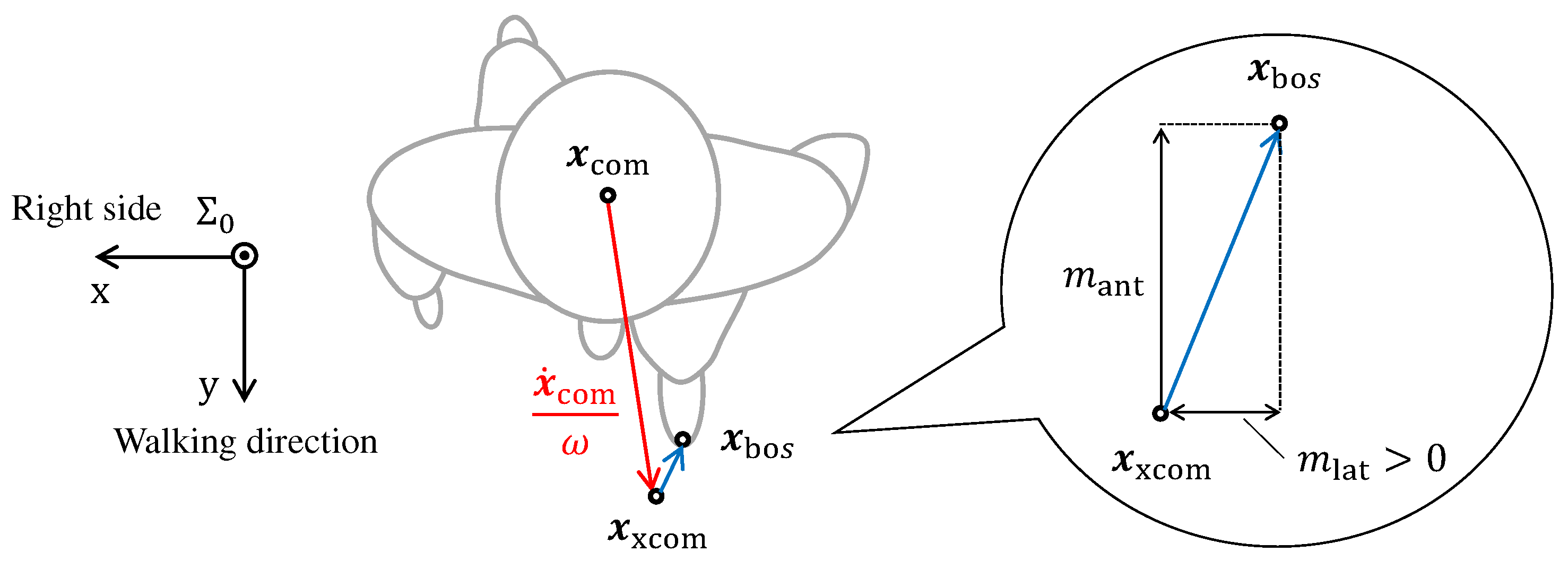
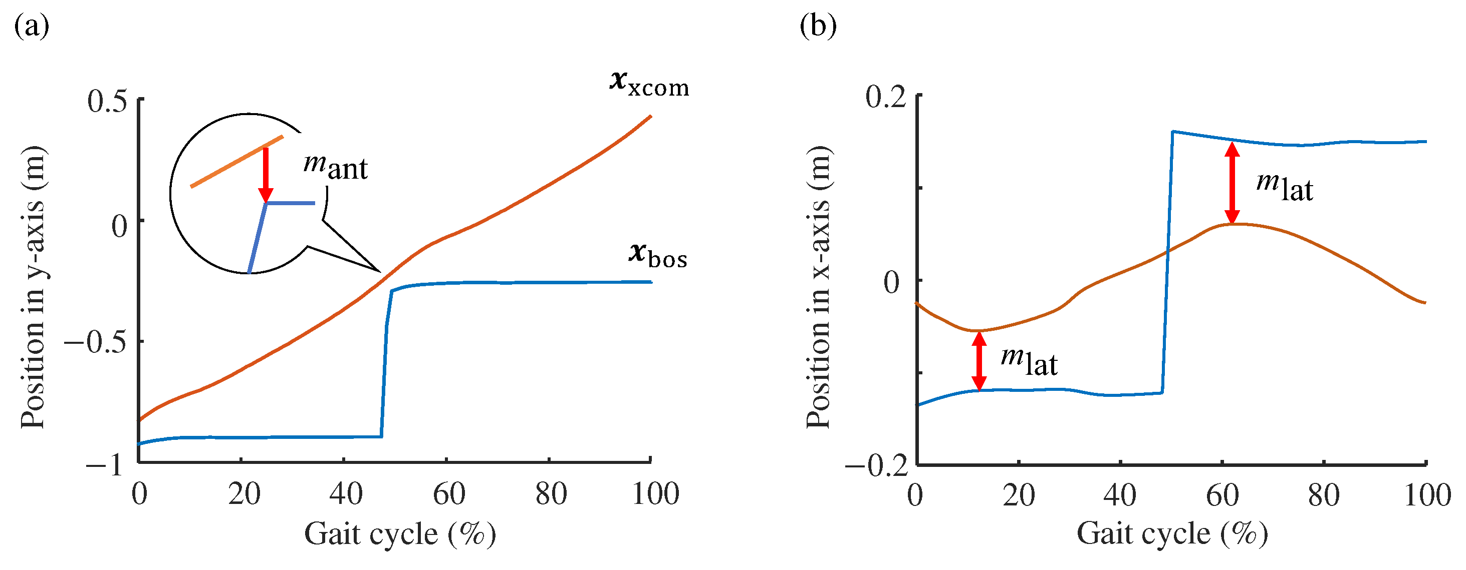
2.2. Computation of Margin of Stability

As shown in Figure 2, the MoS is computed using the position vectors of the center of mass (${\mathit{x}}_{\mathrm{com}}$) and the edge point in the base of the support area (${\mathit{x}}_{\mathrm{bos}}$) in the transverse plane. In this study, ${\mathit{x}}_{\mathrm{com}}$ is the centroid of the right and left anterior superior iliac spines and sacral crest, and ${\mathit{x}}_{\mathrm{bos}}$ is the position of the toe. The distance between these two vectors measures the margin against falling under a still condition. To express the margin during walking, the MoS adopts the concept of an extended center of mass, that is, the position vector of the center of mass prospected in the future [11,12]. The position vector of the extended center of mass is defined as

$$\begin{array}{c}\hfill {\mathit{x}}_{\mathrm{xcom}}={\mathit{x}}_{\mathrm{com}}+{\displaystyle \frac{{\dot{\mathit{x}}}_{\mathrm{com}}}{\omega }},\end{array}$$

(1)

where $\omega$ is the natural angular frequency of an inverted pendulum with a support length of l. The height of the center of body mass corresponds to l. $\omega$ is calculated using l and the gravitational acceleration g:

$$\begin{array}{c}\hfill \omega =\sqrt{{\displaystyle \frac{g}{l}}}.\end{array}$$

(2)

The MoS values for the anterior direction (y) and mediolateral direction (x) are computed separately. The anterior MoS is defined as

$$\begin{array}{c}\hfill m_{\mathrm{ant}}={\mathit{x}}_{\mathrm{bos}}^{\left(y\right)}-{\mathit{x}}_{\mathrm{xcom}}^{\left(y\right)}.\end{array}$$

(3)

Notably, ${\mathit{x}}^{\left(y\right)}$ indicates the y component of vector $\mathit{x}$. Figure 3a shows an example of a change in the extended center of mass (${\mathit{x}}_{\mathrm{xcom}}$) and the endpoint of the base of support (${\mathit{x}}_{\mathrm{bos}}$) during a gait cycle. As a representative value, the most critical moment, which is just after the heel contact, is referred to. Hence, the smaller value between the MoS values at 0% (first heel contact) and ∼50% (second heel contact) is used as the representative MoS value in this study. The anterior MoS value can either be positive or negative. Moreover, the greater the value, the more stable the posture. In the example in the figure, ${\mathit{x}}_{\mathrm{xcom}}$ precedes ${\mathit{x}}_{\mathrm{bos}}$, and the anterior MoS is negative.

The mediolateral MoS is defined as

$$\begin{array}{c}\hfill m_{\mathrm{lat}}=|{\mathit{x}}_{\mathrm{bos}}^{\left(x\right)}-{\mathit{x}}_{\mathrm{xcom}}^{\left(x\right)}|.\end{array}$$

(4)

The mediolateral MoS assumes positive values during normal walking, indicating that the posture remains stable in the mediolateral direction. The value is at a minimum at either ∼10% or ∼60% gait cycle, and the smallest value between them is employed as the most critical value in this study.

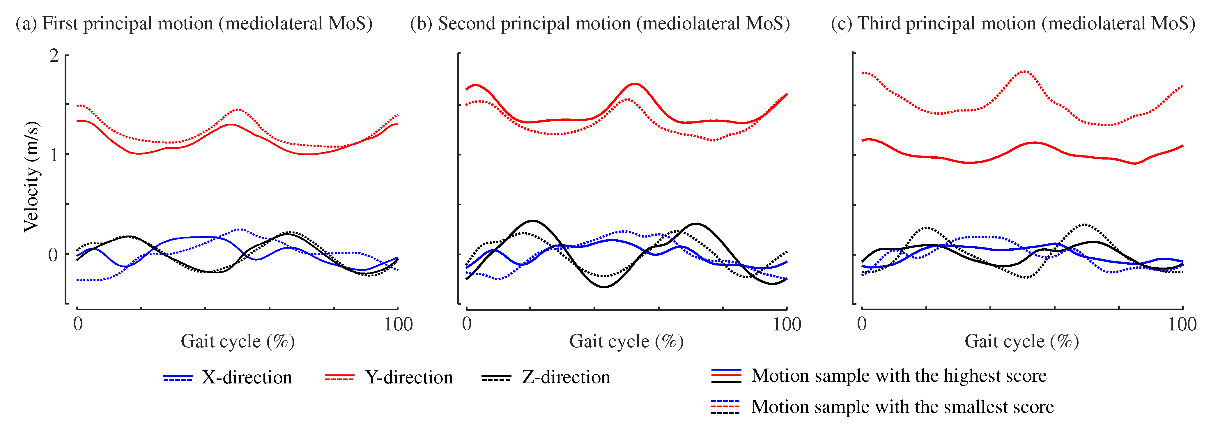
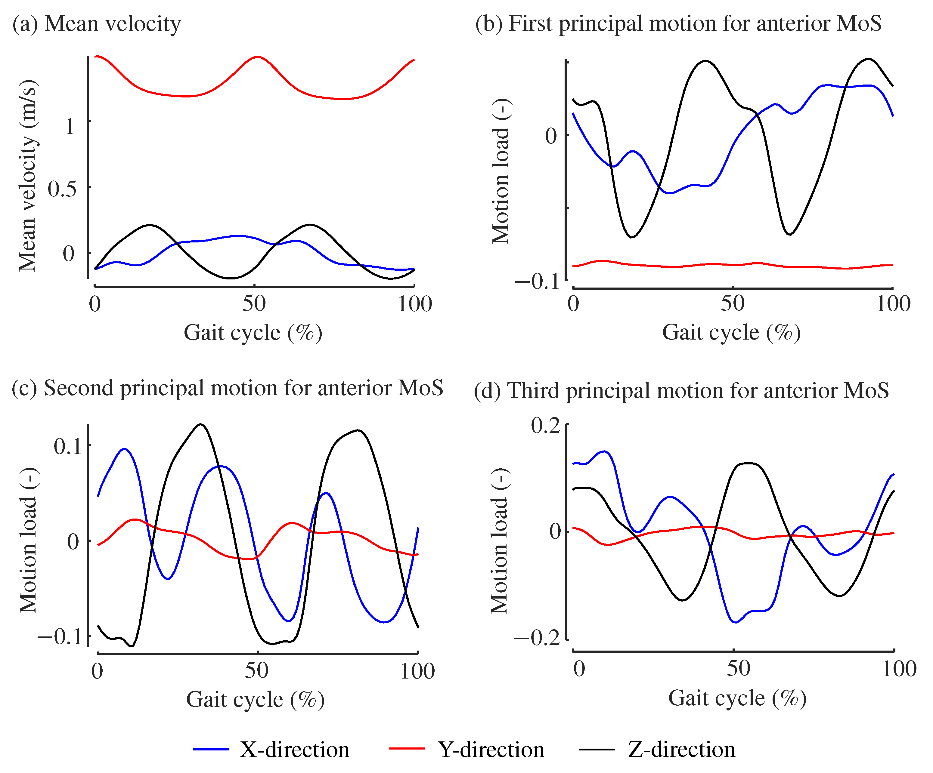
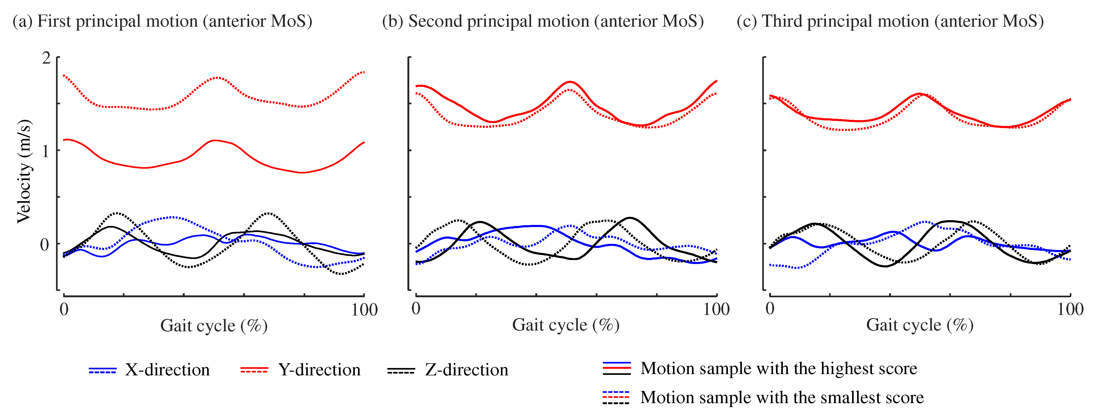
2.3. Principal Motion Analysis to Estimate MoS Values from Kinematic Data

We employ PMA [28] to estimate the MoS values from the triaxial translational velocities of a body feature. PMA encompasses a suite of linear time-series data analysis techniques. It involves decomposing a multidimensional time-series data sample into a set of independent bases, which are also multidimensional time series. The unsupervised variant, known as PMA0, extends the principal component analysis to time-series data and has been applied in the analysis of human motion [35,36,37,38,39]. For this study, we used a supervised variant, PMA1 [28], which is a time-series extension of partial least-squares regression analysis. In PMA1, a time-series data sample is represented as a linear combination of multiple independent time-series bases. These bases are selected to maximize the covariance between the objective variable and principal motion scores, which quantify the extent to which each sample incorporates the bases. Herein, we introduce PMA1 by first explaining partial least-squares regression analysis, followed by the adaptation of its explanatory variables to time-series data.

Let $\mathit{x}\in {\mathbb{R}}^{p\times 1}$ and y be the explanatory vector and objective variable, respectively. ${\mathit{x}}_i$ and $y_i$ are the values from the ith sample ($i=1,\cdots ,n$). These variables are centered such that their mean values are zero: $\overline{\mathit{x}}=\mathbf{0}$ and $\overline{y}=0$. The explanatory vectors of all the samples are displayed in a matrix ($\mathit{X}\in {\mathbb{R}}^{n\times p}$):

$$\begin{array}{c}\hfill \mathit{X}=\left[\begin{array}{c}{\mathit{x}}_1^{\mathrm{T}}\\ ⋮\\ {\mathit{x}}_n^{\mathrm{T}}\end{array}\right].\end{array}$$

(5)

Similarly, the objective values of all the samples are stored in a vector $\mathit{y}\in {\mathbb{R}}^{n\times 1}$:

$$\begin{array}{c}\hfill \mathit{y}={[y_1\cdots y_n]}^{\mathrm{T}}.\end{array}$$

(6)

$\mathit{X}$ and $\mathit{y}$ are approximated as a linear summation of $a^{\prime }$ ($\in \mathbb{N}$) principal components:

$$\begin{array}{c}\hfill \mathit{X}=\sum _{a=1}^{a^{\prime }}{\mathit{t}}_a{\mathit{l}}_a^{\mathrm{T}}+\mathit{E}\end{array}$$

(7)

$$\begin{array}{c}\hfill \mathit{y}=\sum _{a=1}^{a^{\prime }}{b}_a{\mathit{t}}_a+\mathit{e},\end{array}$$

(8)

where ${\mathit{t}}_a\in {\mathbb{R}}^{n\times 1}$ and ${\mathit{l}}_a\in {\mathbb{R}}^{p\times 1}$ are the scores and loadings of the ath principal component ($a=1,\cdots ,a^{\prime }$). $\mathit{E}$ and $\mathit{e}$ are the error matrix and vectors. Let ${\mathit{X}}_a$ and ${\mathit{y}}_a$ be

$$\begin{array}{c}\hfill {\mathit{X}}_a={\mathit{X}}_{a-1}-{\mathit{t}}_{a-1}{\mathit{l}}_{a-1}^{\mathrm{T}}\end{array}$$

(9)

$$\begin{array}{c}\hfill {\mathit{y}}_a={\mathit{y}}_{a-1}-b_{a-1}{\mathit{t}}_{a-1}.\end{array}$$

(10)

Here, ${\mathit{X}}_1=\mathit{X}$ and ${\mathit{y}}_1=\mathit{y}$. ${\mathit{t}}_a$ and ${\mathit{l}}_a$ are computed as

$$\begin{array}{c}\hfill {\mathit{t}}_a={\mathit{X}}_a{\displaystyle \frac{{\mathit{X}}_a^{\mathrm{T}}{\mathit{y}}_a}{|{\mathit{X}}_a^{\mathrm{T}}{\mathit{y}}_a|}}\end{array}$$

(11)

$$\begin{array}{c}\hfill {\mathit{l}}_a={\mathit{X}}_a^{\mathrm{T}}{\displaystyle \frac{{\mathit{t}}_a}{{\mathit{t}}_a^{\mathrm{T}}{\mathit{t}}_a}}\end{array}$$

(12)

$$\begin{array}{c}\hfill b_a={\displaystyle \frac{{\mathit{t}}_a^{\mathrm{T}}}{{\mathit{t}}_a^{\mathrm{T}}{\mathit{t}}_a}}{\mathit{y}}_a,\end{array}$$

(13)

where $|\circ |$ is the L2 norm. $a^{\prime }$ is the number of principal components to approximate the original data and is determined by cross-validation. In this study, $a^{\prime }=3$, which is close to the typical value of two or three for approximating the gait motions of healthy people [26,38,39,40].

To expand the above-mentioned partial least-squares regression to time-series data, $\mathit{x}$ is replaced with a time-series vector. In the case of triaxial kinematic data for gait analysis, each sample includes the translational velocities v along the x, y, and z-directions for one gait cycle, that is, two succeeding steps. The time-series data are discretized by each percentage of the gait cycle. We then acquire

$$\begin{array}{c}\hfill {\mathit{v}}_{\mathit{x}}={[v_{x,0},\cdots ,v_{x,100}]}^{\mathrm{T}}\end{array}$$

(14)

$$\begin{array}{c}\hfill {\mathit{v}}_{\mathit{y}}={[v_{y,0},\cdots ,v_{y,100}]}^{\mathrm{T}}\end{array}$$

(15)

$$\begin{array}{c}\hfill {\mathit{v}}_{\mathit{z}}={[v_{z,0},\cdots ,v_{z,100}]}^{\mathrm{T}}\end{array}$$

(16)

$$\begin{array}{c}\hfill \mathit{x}={\left[{\mathit{v}}_x^{\mathrm{T}}{\mathit{v}}_y^{\mathrm{T}}{\mathit{v}}_z^{\mathrm{T}}\right]}^{\mathrm{T}},\end{array}$$

(17)

where $v_{\{x,y,z\},j}$ is the velocity at j ($\in \{0,1,\cdots ,100\}$) percentage of the gait cycle.

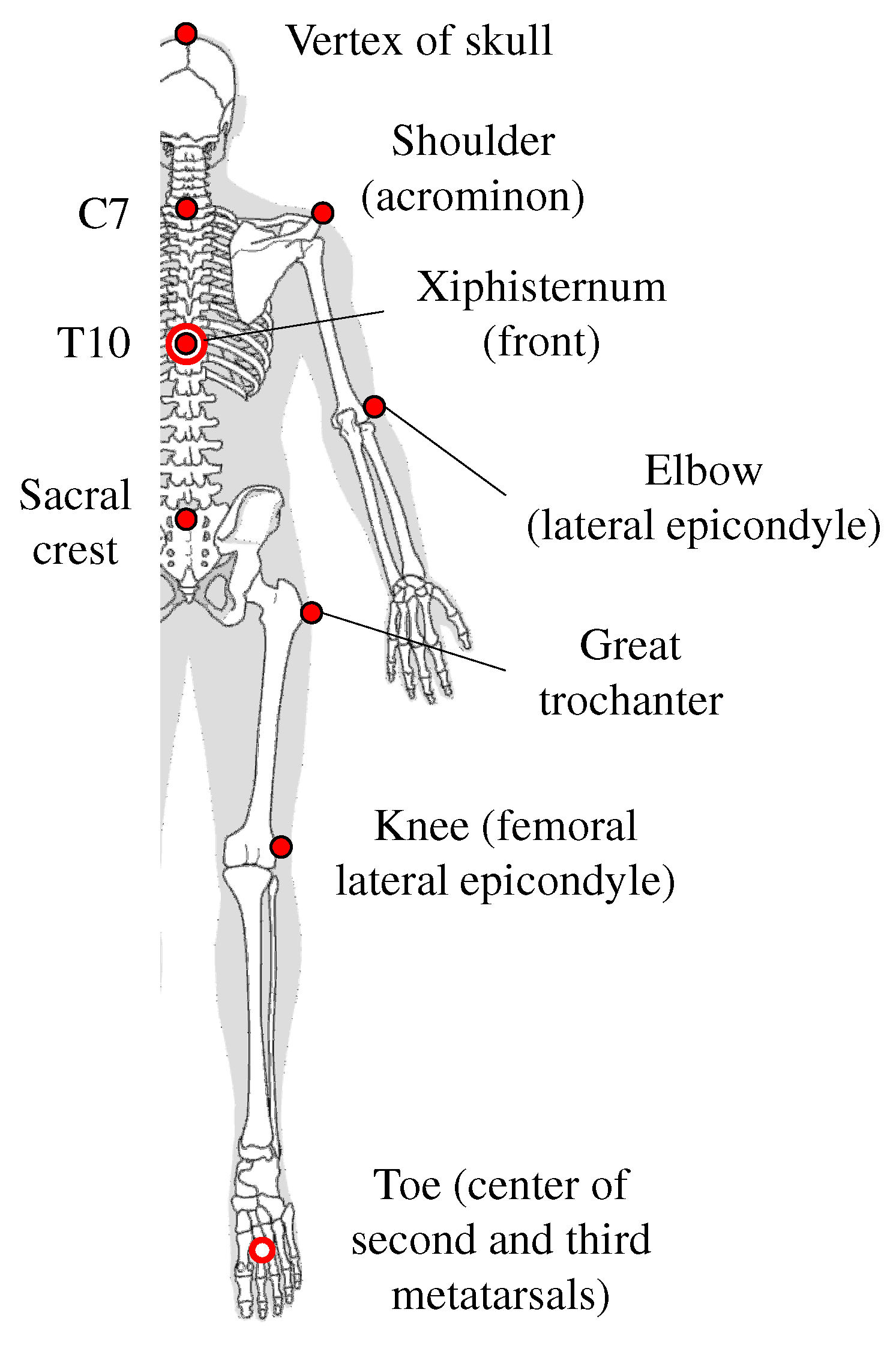
2.4. Comparison of Ten Body Features

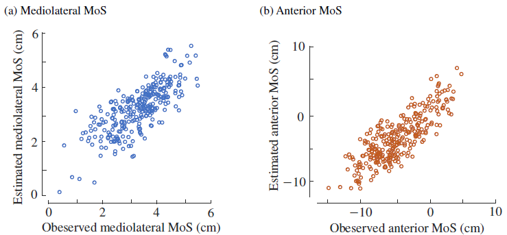
To compare the 10 body features, we calculated PMA1 for both the anterior and mediolateral directions, with the critical MoS values as the objective variables. The explanatory variables were the triaxial velocities of each of the 10 body features described in Section 2.1. We randomly divided 300 samples from 60 individuals into 10 groups, conducting 10-fold cross-validation. Subsequently, we calculated the root mean square errors and correlation coefficients between the estimated MoS values and corresponding observations as performance metrics. Then, the body feature with the highest correlation coefficient was statistically compared to the others. We transformed the correlation coefficients into z values using Fisher’s z transformation [41] and performed paired t-tests for comparison. MATLAB (2023b, Mathworks Inc., Natick, MA, USA) was used for these computations and comparisons. For multiple comparisons, Bonferroni correction of factor nine was adopted to adjust the significance level.

To assess the impact of random bias in the 10-fold cross-validation, we repeated the analysis with different random divisions of samples 20 times. In 18 out of 20 iterations, the same body feature demonstrated the highest performance metrics for both the anterior and mediolateral directions, indicating the robustness of our analysis.

3. Results

Figure 4 shows the mean triaxial velocities of the 10 feature points used for the analysis.

Figure 5 shows the means and standard errors of the correlation coefficients between the observation and prediction of mediolateral and anterior MoS. The values were calculated from the 10 repetitions of cross-validation. Additionally, the figure displays the means and standard errors of the root mean squared errors.

For the mediolateral direction, the sacral crest, knee, and shoulder exhibited the greatest correlation coefficients with $r=0.563$, $0.560$, and $0.558$, respectively. These three features were followed by C7 and T10, with $r=0.508$ and $0.489$, respectively. The lowest correlation coefficient was recorded at the great trochanter and toe with $r=0.330$ and $0.250$, respectively. The correlation coefficients are significantly different among the 10 feature points ($F(9,90)=150.4$, $p<0.001$). The coefficients of the sacral crest that exhibited the highest value were significantly different from those of the seven features: C7 ($t\left(9\right)=7.11$, $p=2.52\times {10}^{-4}$), T10 ($t\left(9\right)=4.91$, $p=3.76\times {10}^{-3}$), elbow ($t\left(9\right)=12.31$, $p=2.79\times {10}^{-6}$), xiphisternum ($t\left(9\right)=17.12$, $p=1.60\times {10}^{-7}$), skull ($t\left(9\right)=8.75$, $p=4.86\times {10}^{-5}$), great trochanter ($t\left(9\right)=14.85$, $p=5.53\times {10}^{-7}$), and toe ($t\left(9\right)=22.18$, $p=1.64\times {10}^{-8}$).

For the anterior direction, the sacral crest exhibited the highest correlation coefficient between the observation and estimation, with $r=0.542$. The sacral crest was followed by the shoulder and knee with $r=0.523$ and 0.518, respectively. The lowest coefficient was exhibited by the toe ($r=0.301$). The coefficients were significantly different among the 10 body features ($F(9,90)=83.2$, $p<0.001$). The correlation coefficient for the sacral crest was significantly greater than those for C7 ($t\left(9\right)=8.57$, $p=5.72\times {10}^{-5}$), T10 ($t\left(9\right)=7.28$, $p=2.10\times {10}^{-4}$), elbow ($t\left(9\right)=20.32$, $p=3.55\times {10}^{-8}$), shoulder ($t\left(9\right)=3.43$, $p=0.034$), xiphisternum ($t\left(9\right)=10.97$, $p=7.41\times {10}^{-6}$), skull ($t\left(9\right)=5.58$, $p=0.0015$), great trochanter ($t\left(9\right)=23.68$, $p<0.001$), and toe ($t\left(9\right)=18.59$, $p<0.001$).

Figure 6 shows the MoS values estimated by cross-validation. Each of these two figures includes 300 points, estimated using 10 different models, with 30 points for each.

Figure 7 shows the mean triaxial velocities of the sacral crest and the first to third principal motions to estimate the mediolateral MoS. As discussed in Section 2.3, each gait sample is represented as a linear combination of these three principal motions with the principal motion scores (${\mathit{t}}_a$) indicating the contribution of each motion. Notably, all samples were normalized to have $\overline{\mathit{x}}=\mathbf{0}$, and the principal motions highlight the deviations from the mean motions. The estimation of the mediolateral MoS for the sacral crest involves the sum of the three principal motion scores:

$$\begin{array}{c}\hfill {\mathit{m}}_{\mathrm{lat}}=0.160{\mathit{t}}_1+0.0488{\mathit{t}}_2+0.0457{\mathit{t}}_3+{\overline{m}}_{\mathrm{lat}},\end{array}$$

(18)

where ${\overline{m}}_{\mathrm{lat}}$ is the mean mediolateral MoS value across all samples. As shown in Figure 7b, the characteristic movement of the first principal motion is along the x-axis. On average, as shown in Figure 7a, the x-direction velocity reaches its minimum and maximum at approximately 0% and 50% of the gait cycle, respectively. Conversely, the load distribution of the first principal motion demonstrates almost opposite characteristics, with maximum and minimum values at roughly 0% and 50% of the gait cycle, respectively. This pattern suggests that individuals with higher first scores exhibit less variation in the x-direction velocity. This observation is further supported by Figure 8a, where gait samples with the highest and lowest first scores are depicted with solid and dotted lines, respectively. Notably, the higher the score, the higher the MoS value and postural stability. The extended center of mass becomes close to the center of the body with low speeds in the x-direction, implying a high postural stability. Therefore, individuals with high first scores and minimal fluctuation in the x-directional speed tend to have large mediolateral MoS values. Figure 7c shows that the dominant feature of the second principal motion is along the z-axis, lagging behind the mean motion by approximately 10%. This delay suggests that individuals with elevated second scores experience delayed peaks in the z-directional velocities, as shown in Figure 8b. Similarly, Figure 7d and Figure 8c show that the defining characteristic of the third principal motion is a reduced walking speed (y-directional velocity), with individuals exhibiting large third scores when walking slowly, probably because of the short strides, as indicated by the reduced vertical movement.

Figure 9 shows the mean translational velocities of the sacral crest and the first to third principal motions for estimating the anterior MoS. The anterior MoS for the sacral crest was estimated by summing the following three principal motion scores:

$$\begin{array}{c}\hfill {\mathit{m}}_{\mathrm{ant}}=0.0792{\mathit{t}}_1+0.0480{\mathit{t}}_2+0.0432{\mathit{t}}_3+{\overline{m}}_{\mathrm{ant}},\end{array}$$

(19)

where ${\overline{m}}_{\mathrm{ant}}$ represents the mean anterior MoS value across all samples. Figure 10 compares motion samples with the highest (represented by solid curves) and smallest (represented by dotted curves) scores for each principal motion. Figure 9b shows that the prominent feature of the first principal motion is small velocities in the y-direction, with velocities in the x- and z-directions approximately in the opposite phase to the average motions. Consequently, as shown in Figure 10a, participants with a large first score walk slowly with small velocity amplitudes in the mediolateral (x) and vertical (z) directions, indicating a gait with small strides. The second principal motion is characterized by a lag in the z-direction velocity, as shown in Figure 9c and Figure 10b. A motion sample with a large second score shows a delay in the z-direction phase. Figure 9d and Figure 10c show noticeable differences in motions between large and small third scores, particularly in the x- and z-directions. Compared with the sample with a small score, the sample with a large score advances in phase in the z-direction. Additionally, the sample with a large score exhibits minimal change in the x-directional velocity.

4. Discussion

As shown in Section 3, the kinematic information from the sacral crest and knee can most accurately estimate both the anterior and mediolateral MoSs. The sacral crest was anticipated to be a suitable estimation point owing to its proximity to the center of body mass (${\mathit{x}}_{\mathrm{com}}$), which is used for MoS calculations. Further, the positions of the feet can be accurately predicted using the motion of the center of mass [42,43], implying that only the kinematic information near the center of mass is satisfactory to predict the MoSs. Following the sacral crest, the xiphisternum, T10 vertebra, and great trochanter are the feature points closest to the center of body mass. However, the estimation accuracies for the xiphisternum and T10 did not match that of the sacral crest. This discrepancy could be attributed to the separation of the xiphisternum and T10 from the center of body mass by several spinal and coastal bones, potentially weakening their motion correlation with the sacral crest. The great trochanter, despite its proximity to the center of body mass, proved to be the least suitable point for MoS estimation, similar to the toe. This may be because the femur, prominently featuring the great trochanter, moves independently from the pelvis, which comprises the sacral crest, rendering it less relevant for MoS estimations. Contrarily, the femoral lateral epicondyle, another prominent feature of the femur, achieved estimation accuracies comparable to the sacral crest. A possible explanation for this is that the great trochanter is located near the instant center of rotation of the femur [44], where its translational motion is minimal and hence less contributory to MoS estimation.

The knee, along with the sacral crest, was identified as a suitable point for estimating the MoS. This suitability may stem from the position of the knee, which captures motion information from both the center of body mass and toe, as it is located between them. In healthy individuals, the knee is almost fully extended at the moment of heel contact [45], rendering its motion information valuable for predicting foot position. The position marker of the knee, attached to the femoral lateral epicondyle, does not capture information regarding the abduction and adduction movements of the knee joint. However, unexpectedly, the knee also proved effective for estimating the mediolateral MoS. This finding necessitates further investigation to elucidate the underlying mechanisms in future studies.

The toe was unsuitable, although it is used for computing the MoS. This is potentially because the toe does not include significant kinematic information during the stance phase. As shown in Figure 4j, the right toe rarely moves for approximately 40% of the gait cycle. Notably, the typical stance phase occupies 60% of the gait cycle [46,47], but the toe continues to move immediately after the heel contact. Further, during the swing phase, the ankle joint can move freely in the air or at least without the restriction caused by the contact with the ground, although such motions are used to determine the toe clearance [48,49,50]. Ankle motions in the air may not be directly linked to the MoS that is computed referring to the foot position during the stance phase. Collectively, the toe is reasonably judged as an unsuitable point to estimate the MoS.

This study identifies two body points—the sacral crest and knee—as suitable for estimating the anterior and mediolateral MoSs based on their kinematic information. When attaching the IMUs to these points using a cloth bandage, areas near joints where the attachment may loosen during extended periods of walking should be avoided. In practice, IMUs are typically affixed near the knee, either on the femoral or tibial parts [10,51,52,53]. Considering these practical considerations for fixation, further research is needed to refine our understanding and approach.

The accuracy of MoS estimation requires further enhancement, although specific criteria have not been established in this study. We propose two potential strategies for improvement. First, considering that MoS values can also be estimated from the angular velocities of the pelvis [27], integrating angular and translational velocities might enhance accuracy. Second, employing multiple IMUs could increase the accuracy. With IMUs now commonly incorporated into smartphones and smartwatches, it is feasible that individuals might carry two IMU-equipped devices in their daily lives. Future research will explore the optimal locations for attaching these two IMUs.

A limitation of this study is our reliance on optical motion capture systems rather than IMUs to collect body motion data. Although IMUs are recognized as potential alternatives to optical systems [10,54,55,56], they may entail a loss of accuracy. A challenge with IMU usage concerns securing them to the body effectively. Because of their inertia, including the weight of batteries and communication devices, IMUs may exacerbate noise issues associated with soft tissue movements beneath skin, in contrast to the lightweight reflective markers used in optical systems [57]. Another consideration is the calculation of the center of mass. We approximated the center of mass of the body using the geometric center of three pelvis points because of the lack of inertial data for body segments. This approximation is close to the true center of body mass [58] and is deemed acceptable for MoS calculations. However, this study specifically associates the center of mass with the sacral crest, potentially leading to an overestimation of its effectiveness in MoS estimation. To address these issues and validate the feasibility of IMU-based MoS estimations, future studies should involve experiments that concurrently use optical motion capture systems and IMUs. The definitive potential of IMUs for MoS estimation can be confirmed by further experimental investigations.

5. Conclusions

We investigated suitable body points for estimating the anterior and mediolateral MoSs from triaxial translational velocities, assuming the use of an IMU, such as those installed in smartphones. To the best of our knowledge, no previous studies have reported similar findings. Among the 10 points evaluated, the sacral crest and knee were identified as the most accurate for MoS estimation. When using the sacral crest, the mean correlation coefficients between the estimated and observed MoSs were 0.563 for the mediolateral direction and 0.542 for the anterior direction, respectively. For the knee, these coefficients were 0.560 and 0.518, respectively. These two features are considered as promising points to attach IMUs. Future research will explore the feasibility of IMU-based MoS estimation as a method for accessible MoS measurement in everyday life. Our findings pave the way for developing an accessible system to estimate fall risks.

References

1. Balance Augmentation in Locomotion, through Anticipative, Natural and Cooperative Control of Exoskeletons; Report of BALANCE-Deliverable 3.1-Stability index 2013; European Commision: Brussels, Belgium, 2013.
2. Bruijn, S.; Meijer, O.; Beek, P.; van Dieën, J. Assessing the stability of human locomotion: A review of current measures. J. R. Soc. Interface 2013, 10, 20120999. [Google Scholar] [CrossRef]
3. Gillespie, L.D.; Robertson, M.C.; Gillespie, W.J.; Sherrington, C.; Gates, S.; Clemson, L.; Lamb, S.E. Interventions for preventing falls in older people living in the community. Cochrane Database Syst. Rev. 2012, 2021, CD007146. [Google Scholar] [CrossRef]
4. Kim, Y.K.; Joo, J.Y.; Jeong, S.H.; Jeon, J.H.; Jung, D.Y. Effects of walking speed and age on the directional stride regularity and gait variability in treadmill walking. J. Mech. Sci. Technol. 2016, 30, 2899–2906. [Google Scholar] [CrossRef]
5. Liu, T.; Inoue, Y.; Shibata, K. Development of a wearable sensor system for quantitative gait analysis. Measurement 2009, 42, 978–988. [Google Scholar] [CrossRef]
6. Jebelli, H.; Ahn, C.R.; Stentz, T.L. Comprehensive Fall-Risk Assessment of Construction Workers Using Inertial Measurement Units: Validation of the Gait-Stability Metric to Assess the Fall Risk of Iron Workers. J. Comput. Civ. Eng. 2016, 30, 04015034. [Google Scholar] [CrossRef]
7. Mariani, B.; Hoskovec, C.; Rochat, S.; Büla, C.; Penders, J.; Aminian, K. 3D gait assessment in young and elderly subjects using foot-worn inertial sensors. J. Biomech. 2010, 43, 2999–3006. [Google Scholar] [CrossRef] [PubMed]
8. Jebelli, H.; Ahn, C.R.; Stentz, T.L. Fall risk analysis of construction workers using inertial measurement units: Validating the usefulness of the postural stability metrics in construction. Saf. Sci. 2016, 84, 161–170. [Google Scholar] [CrossRef]
9. Yang, K.; Ahn, C.R.; Vuran, M.C.; Aria, S.S. Semi-supervised near-miss fall detection for ironworkers with a wearable inertial measurement unit. Autom. Constr. 2016, 68, 194–202. [Google Scholar] [CrossRef]
10. Riek, P.M.; Best, A.N.; Wu, A.R. Validation of Inertial Sensors to Evaluate Gait Stability. Sensors 2023, 23, 1547. [Google Scholar] [CrossRef]
11. Hof, A.; Gazendam, M.; Sinke, W. The condition for dynamic stability. J. Biomech. 2005, 38, 1–8. [Google Scholar] [CrossRef]
12. Hof, A.L. The ‘extrapolated center of mass’ concept suggests a simple control of balance in walking. Hum. Mov. Sci. 2008, 27, 112–125. [Google Scholar] [CrossRef]
13. Watson, F.; Fino, P.C.; Thornton, M.; Heracleous, C.; Loureiro, R.; Leong, J.J.H. Use of the margin of stability to quantify stability in pathologic gait—A qualitative systematic review. BMC Musculoskelet. Disord. 2021, 22, 597. [Google Scholar] [CrossRef]
14. Akiyama, Y.; Kuboki, Y.; Okamoto, S.; Yamada, Y. Novel Approach to Analyze All-Round Kinematic Stability during Curving Steps. IEEE Access 2023, 11, 10326–10335. [Google Scholar] [CrossRef]
15. Ohtsu, H.; Yoshida, S.; Minamisawa, T.; Takahashi, T.; Yomogida, S.i.; Kanzaki, H. Investigation of balance strategy over gait cycle based on margin of stability. J. Biomech. 2019, 95, 109319. [Google Scholar] [CrossRef] [PubMed]
16. Harro, C.; Alderink, G.; Hickox, L.; Zeitler, D.W.; Avery, M.; Daman, C.; Laker, D. Dynamic Measures of Balance during Obstacle-Crossing in Self-Selected Gait in Individuals with Mild-to-Moderate Parkinson’s Disease. Appl. Sci. 2024, 14, 1271. [Google Scholar] [CrossRef]
17. Kuroda, T.; Okamoto, S.; Akiyama, Y. Anterior and mediolateral dynamic gait stabilities attributed to different gait parameters in different age groups. J. Biomech. Sci. Eng. 2024, 19, 23–00183. [Google Scholar] [CrossRef]
18. Nagano, H. Gait Biomechanics for Fall Prevention among Older Adults. Appl. Sci. 2022, 12, 6660. [Google Scholar] [CrossRef]
19. Fallahtafti, F.; Bruijn, S.; Mohammadzadeh Gonabadi, A.; Sangtarashan, M.; Boron, J.B.; Curtze, C.; Siu, K.C.; Myers, S.A.; Yentes, J. Trunk Velocity Changes in Response to Physical Perturbations Are Potential Indicators of Gait Stability. Sensors 2023, 23, 2833. [Google Scholar] [CrossRef]
20. Akiyama, Y.; Fukui, Y.; Okamoto, S.; Yamada, Y. Effects of exoskeletal gait assistance on the recovery motion following tripping. PLoS ONE 2020, 15, e0229150. [Google Scholar] [CrossRef] [PubMed]
21. Alderink, G.; Harro, C.; Hickox, L.; Zeitler, D.W.; Bourke, M.; Gosla, A.; Rustmann, S. Dynamic Measures of Balance during a 90° Turn in Self-Selected Gait in Individuals with Mild Parkinson’s Disease. Appl. Sci. 2023, 13, 5428. [Google Scholar] [CrossRef]
22. Varas-Diaz, G.; Jayakumar, U.; Taras, B.; Wang, S.; Bhatt, T. Assessing Balance Loss and Stability Control in Older Adults Exposed to Gait Perturbations under Different Environmental Conditions: A Feasibility Study. Biomechanics 2022, 2, 374–394. [Google Scholar] [CrossRef]
23. Hak, L.; Hettinga, F.J.; Duffy, K.R.; Jackson, J.; Sandercock, G.R.; Taylor, M.J. The concept of margins of stability can be used to better understand a change in obstacle crossing strategy with an increase in age. J. Biomech. 2019, 84, 147–152. [Google Scholar] [CrossRef] [PubMed]
24. Park, S.; Ko, Y.M.; Park, J.W. The Correlation between Dynamic Balance Measures and Stance Sub-phase COP Displacement Time in Older Adults during Obstacle Crossing. J. Phys. Ther. Sci. 2013, 25, 1193–1196. [Google Scholar] [CrossRef] [PubMed]
25. Sivakumaran, S.; Schinkel-Ivy, A.; Masani, K.; Mansfield, A. Relationship between margin of stability and deviations in spatiotemporal gait features in healthy young adults. Hum. Mov. Sci. 2018, 57, 366–373. [Google Scholar] [CrossRef] [PubMed]
26. Iwasaki, T.; Okamoto, S.; Akiyama, Y.; Yamada, Y. Gait Stability Index Built by Kinematic Information Consistent with the Margin of Stability along the Mediolateral Direction. IEEE Access 2022, 10, 52832–52839. [Google Scholar] [CrossRef]
27. Liu, Z.; Kuroda, T.; Okamoto, S.; Akiyama, Y. Estimation of Mediolateral Gait Postural Stability using Time-Series Pelvis Angular Velocities. In Proceedings of the IEEE Global Conference on Consumer Electronics, Osaka, Japan, 18–21 October 2022; pp. 754–756. [Google Scholar] [CrossRef]
28. Qiu, C.; Okamoto, S.; Akiyama, Y.; Yamada, Y. Application of Supervised Principal Motion Analysis to Evaluate Subjectively Easy Sit-to-Stand Motion of Healthy People. IEEE Access 2021, 9, 73251–73261. [Google Scholar] [CrossRef]
29. Liu, Z.; Kuroda, T.; Okamoto, S.; Akiyama, Y. Suitability of Sacrum Motion in Computing Dynamic Gait Stability Indices. In Proceedings of the IEEE Global Conference on Consumer Electronics, Nara, Japan, 10–13 October 2023; pp. 343–345. [Google Scholar] [CrossRef]
30. Kobayashi, Y.; Hida, N.; Nakajima, K.; Fujimoto, M.; Mochimaru, M. AIST Gait Database 2019. Available online: https://unit.aist.go.jp/harc/ExPART/GDB2019.html (accessed on 1 June 2019).
31. Yamaguchi, T.; Masani, K. Effects of age on dynamic balance measures and their correlation during walking across the adult lifespan. Sci. Rep. 2022, 12, 14301. [Google Scholar] [CrossRef] [PubMed]
32. Hiyama, T.; Kobayashi, Y.; Matsumoto, Y.; Murai, A.; Fujimoto, M.; Ozawa, J.; Mochimaru, M. Comparison of Machine Learning Methods and Gait Characteristics for Classification of Fallers and Non-fallers. Adv. Biomed. Eng. 2023, 12, 182–192. [Google Scholar] [CrossRef]
33. Slijepcevic, D.; Horst, F.; Simak, M.; Lapuschkin, S.; Raberger, A.; Samek, W.; Breiteneder, C.; Schöllhorn, W.; Zeppelzauer, M.; Horsak, B. Explaining machine learning models for age classification in human gait analysis. Gait Posture 2022, 97, S252–S253. [Google Scholar] [CrossRef]
34. Faul, F.; Erdfelder, E.; Lang, A.G.; Buchner, A. G*Power 3: A flexible statistical power analysis program for the social, behavioral, and biomedical sciences. Behav. Res. Methods 2007, 39, 175–191. [Google Scholar] [CrossRef]
35. Park, F.C.; Jo, K. Movement Primitives and Principal Component Analysis. In Proceedings of the on Advances in Robot Kinematics; Lenarčič, J., Galletti, C., Eds.; Springer: Dordrecht, The Netherlands, 2004; pp. 421–430. [Google Scholar]
36. Lim, B.; Ra, S.; Park, F.C. Movement Primitives, Principal Component Analysis, and the Efficient Generation of Natural Motions. In Proceedings of the Proceedings of the 2005 IEEE International Conference on Robotics and Automation, Barcelona, Spain, 18–22 April 2005; pp. 4630–4635. [Google Scholar] [CrossRef]
37. St-Onge, N.; Feldman, A.G. Interjoint coordination in lower limbs during different movements in humans. Exp. Brain Res. 2003, 148, 139–149. [Google Scholar] [CrossRef] [PubMed]
38. Borghese, N.A.; Bianchi, L.; Lacquaniti, F. Kinematic determinants of human locomotion. J. Physiol. 1996, 494, 863–879. [Google Scholar] [CrossRef] [PubMed]
39. Mah, C.D.; Hulliger, M.; Lee, R.G.; O’Callaghan, I.S. Quantitative Analysis of Human Movement Synergies: Constructive Pattern Analysis for Gait. J. Mot. Behav. 1994, 26, 83–102. [Google Scholar] [CrossRef]
40. Funato, T.; Aoi, S.; Oshima, H.; Tsuchiya, K. Variant and invariant patterns embedded in human locomotion through whole body kinematic coordination. Exp. Brain Res. 2010, 205, 497–511. [Google Scholar] [CrossRef] [PubMed]
41. Hotelling, H. New Light on the Correlation Coefficient and its Transforms. J. R. Stat. Soc. Ser. (Methodol.) 1953, 15, 193–225. [Google Scholar] [CrossRef]
42. Vlutters, M.; Van Asseldonk, E.; Van der Kooij, H. Center of mass velocity based predictions in balance recovery following pelvis perturbations during human walking. J. Exp. Biol. 2016, 219, 1514–1523. [Google Scholar] [CrossRef]
43. Wang, Y.; Srinivasan, M. Stepping in the direction of the fall: The next foot placement can be predicted from current upper body state in steady-state walking. Biol. Lett. 2014, 10, 20140405. [Google Scholar] [CrossRef] [PubMed]
44. Crenna, F.; Rossi, G.B.; Palazzo, A. Instantaneous centre of rotation in human motion: Measurement and computational issues. J. Phys. Conf. Ser. 2016, 772, 012027. [Google Scholar] [CrossRef]
45. Scanlan, S.F.; Favre, J.; Andriacchi, T.P. The relationship between peak knee extension at heel-strike of walking and the location of thickest femoral cartilage in ACL reconstructed and healthy contralateral knees. J. Biomech. 2013, 46, 849–854. [Google Scholar] [CrossRef]
46. Whittle, M.W. Clinical gait analysis: A review. Hum. Mov. Sci. 1996, 15, 369–387. [Google Scholar] [CrossRef]
47. Kharb, A.; Saini, V.; Jain, Y.; Dhiman, S. A review of gait cycle and its parameters. Int. J. Comput. Eng. Manag. 2011, 13, 78–83. [Google Scholar]
48. Mills, P.M.; Barrett, R.S. Swing phase mechanics of healthy young and elderly men. Hum. Mov. Sci. 2001, 20, 427–446. [Google Scholar] [CrossRef] [PubMed]
49. Schulz, B.W. A new measure of trip risk integrating minimum foot clearance and dynamic stability across the swing phase of gait. J. Biomech. 2017, 55, 107–112. [Google Scholar] [CrossRef] [PubMed]
50. Ullauri, J.B.; Akiyama, Y.; Okamoto, S.; Yamada, Y. Technique to reduce the minimum toe clearance of young adults during walking to simulate the risk of tripping of the elderly. PLoS ONE 2019, 14, e0217336. [Google Scholar] [CrossRef] [PubMed]
51. Mavor, M.P.; Ross, G.B.; Clouthier, A.L.; Karakolis, T.; Graham, R.B. Validation of an IMU Suit for Military-Based Tasks. Sensors 2020, 20, 4280. [Google Scholar] [CrossRef] [PubMed]
52. Antunes, R.; Jacob, P.; Meyer, A.; Conditt, M.A.; Roche, M.W.; Verstraete, M.A. Accuracy of Measuring Knee Flexion after TKA through Wearable IMU Sensors. J. Funct. Morphol. Kinesiol. 2021, 6, 60. [Google Scholar] [CrossRef] [PubMed]
53. Drapeaux, A.; Carlson, K. A Comparison of Inertial Motion Capture Systems: DorsaVi and Xsens. Int. J. Kinesiol. Sport. Sci. 2020, 8, 24. [Google Scholar] [CrossRef]
54. Teufl, W.; Lorenz, M.; Miezal, M.; Taetz, B.; Fröhlich, M.; Bleser, G. Towards Inertial Sensor Based Mobile Gait Analysis: Event-Detection and Spatio-Temporal Parameters. Sensors 2019, 19, 38. [Google Scholar] [CrossRef]
55. Schwesig, R.; Leuchte, S.; Fischer, D.; Ullmann, R.; Kluttig, A. Inertial sensor based reference gait data for healthy subjects. Gait Posture 2011, 33, 673–678. [Google Scholar] [CrossRef]
56. Ciklacandir, S.; Ozkan, S.; Isler, Y. A Comparison of the Performances of Video-Based and IMU Sensor-Based Motion Capture Systems on Joint Angles. In Proceedings of the 2022 Innovations in Intelligent Systems and Applications Conference (ASYU), Antalya, Turkey, 7–9 September 2022; pp. 1–5. [Google Scholar] [CrossRef]
57. Cockcroft, J.; Louw, Q.; Baker, R. Proximal placement of lateral thigh skin markers reduces soft tissue artefact during normal gait using the Conventional Gait Model. Comput. Methods Biomech. Biomed. Eng. 2016, 19, 1497–1504. [Google Scholar] [CrossRef]
58. WS, E. Center of mass of the human body helps in analysis of balance and movement. MOJ Appl. Bionics Biomech. 2018, 2, 144–148. [Google Scholar] [CrossRef]
Figure 1. Feature points examined in the study. Open circles indicate the feature points on the frontal side.
Applsci 14 03067 g001
Figure 2. Margin of stability. Top view of a walking person.
Applsci 14 03067 g002
Figure 3. Margin of stability and changes in the extended center of mass and base of support. (a) Y-direction (anterior) and (b) X-direction (mediolateral).
Applsci 14 03067 g003
Figure 4. Mean translational velocities of 10 feature points during a gait cycle. (a) Skull, (b) T10, (c) right shoulder, (d) sacral crest, (e) xiphisternum, (f) C7, (g) right elbow, (h) right great trochanter, (i) right knee, and (j) right toe.
Applsci 14 03067 g004
Figure 5. Means and standard errors of correlation coefficients and root mean squared errors between estimated and observed MoS values. (a) Mediolateral and (b) anterior MoS values. *, ** and *** indicate significant difference at p < 0.05 , 0.01, and 0.001, respectively, by paired t-tests with Bonferroni correction of factor nine.
Applsci 14 03067 g005
Figure 6. Observed and estimated MoS. (a) Mediolateral direction and (b) anterior direction. MoS values were estimated by 10-fold cross-validation.
Applsci 14 03067 g006
Figure 7. Mean translational velocities of the sacral crest and principal motions to estimate the mediolateral MoS. (a) Mean translational velocities. (b) First principal motion. (c) Second principal motion. (d) Third principal motion.
Applsci 14 03067 g007
Figure 8. Examples of gait motions with the highest (rigid curves) and smallest (dotted curves) scores for each principal motion to estimate the mediolateral MoS.
Applsci 14 03067 g008
Figure 9. Mean translational velocities of the sacral crest and principal motions to estimate the anterior MoS. (a) Mean translational velocities (same as Figure 7a). (b) First principal motion. (c) Second principal motion. (d) Third principal motion.
Applsci 14 03067 g009
Figure 10. Examples of gait motions with the highest (rigid curves) and smallest (dotted curves) scores for each principal motion to estimate the anterior MoS.
Applsci 14 03067 g010
Disclaimer/Publisher’s Note: The statements, opinions and data contained in all publications are solely those of the individual author(s) and contributor(s) and not of MDPI and/or the editor(s). MDPI and/or the editor(s) disclaim responsibility for any injury to people or property resulting from any ideas, methods, instructions or products referred to in the content.