Study on Oscillatory and Undulatory Motion of Robotic Fish

Abstract

This paper conducts a comprehensive analysis of undulating and oscillatory movements in fish, utilizing numerical simulations to explore correlations among fin thrust and swimming speed. The study distinguishes itself through a unique approach by employing kinematic equations of motion control, specifically in oscillation and undulation, for computational fluid dynamics. Despite increasing energy loss with undulation, the study reveals a reduction in power demand with oscillation, underscoring its effectiveness in achieving desired speeds. The dynamics of undulating fins in aquatic and aerial locomotion remain insufficiently understood. The trade-off between more energy-consuming but highly propulsive movements or simpler and faster movements requires sophisticated design techniques to reduce volume. The geometry, developed using Rhino 6 software, incorporates precise fluid resistance calculations conducted with Ansys Fluent 19. Spanning flow velocities from 1 to 4 m/s were used for the simulation condition. Critical factors such as flexibility, viscosity, and shape change were meticulously examined for their impact on efficiency enhancement.

1. Introduction

The ocean is a vital source of resources for society, with the demand for seawater, minerals, and biological resources surpassing that of land. The scientific community aims to explore and utilize the ocean safely and effectively [1]. Modern multipurpose submersibles can operate at various depths, from shallow to oceanic. New development goals focus on optimizing performance, addressing complex hydrodynamic effects like swimming and noise control, drawing inspiration from underwater animals [2]. In contrast to traditional submarines, fish have evolved to use oscillatory motions, providing high thrust, excellent maneuverability, and low noise levels in the flow field. The study also illustrates the ability of aquatic animals to sense complex underwater environments. Research in fish biology, inspired by nature and the design of fish robots, plays a crucial role in developing the next generation of submarines [3,4].

While extensive research has been conducted in related fields, numerous scientific and technological challenges persist. Computational fluid dynamics (CFDs) serve as a key tool to bolster experimental research but face notable issues, particularly the demand for substantial computational resources [5]. The fish’s propulsion ability arises from the coordinated action of muscle groups, facilitating even weight distribution across the body and an efficient movement structure that conserves space. These fluid recognition systems empower aluminum foils to discern turbulence information within the flow field, effectively harnessing energy to enhance efficiency. In conventional simulation studies, the observation of vortex shedding in fluid flow often involves a simplified representation of stationary objects due to the intricate nature of fluid dynamics [6]. However, in this particular investigation, a novel approach is taken, where the fluid flow is simulated through a dynamically moving object. This unique methodology aims to provide insights into and support the design of the streamlined shape for robotic fish.

Swimming, a phenomenon deeply ingrained in the evolutionary tapestry of nature, continues to captivate the scientific and engineering communities [7,8]. Fish swimming, in particular, has been a subject of keen interest, offering profound insights into the optimization of underwater vehicles and biomimetic robots. The kinematic equation of motion is a key focus area, where advanced equations of motion control, particularly in oscillation and undulation, are leveraged to conduct fluid dynamics calculations. This approach aims to unravel the underlying physics governing fish movements [9,10]. This interdisciplinary exploration promises to provide valuable insights into the fluid dynamics and kinematics of fish-inspired swimming. The knowledge gained has the potential to impact the optimization of underwater vehicles and inspire advancements in biomimetic robotic systems. This research embarks on a computational journey to explore the intricacies of fish-inspired swimming, focusing on two fundamental forms of motion: undulatory and oscillatory. The aims of this study are as follows:

–

Utilize the equations of motion control (oscillation and undulation) for fluid dynamic calculations.

–

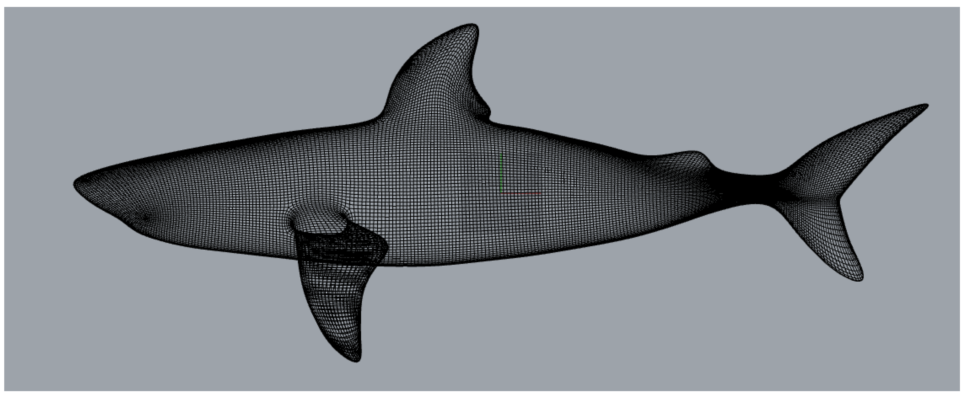
Develop the model’s shape and control the movement approach to aid in reaching the desired fish swimming at high speed.

The rest of this paper is organized as follows: mathematical modeling of the oscillatory and undulatory motion is presented in Section 2; computer simulation of the drag force of the fish model is presented in Section 3; and conclusions are presented in Section 4.

2. Methodology

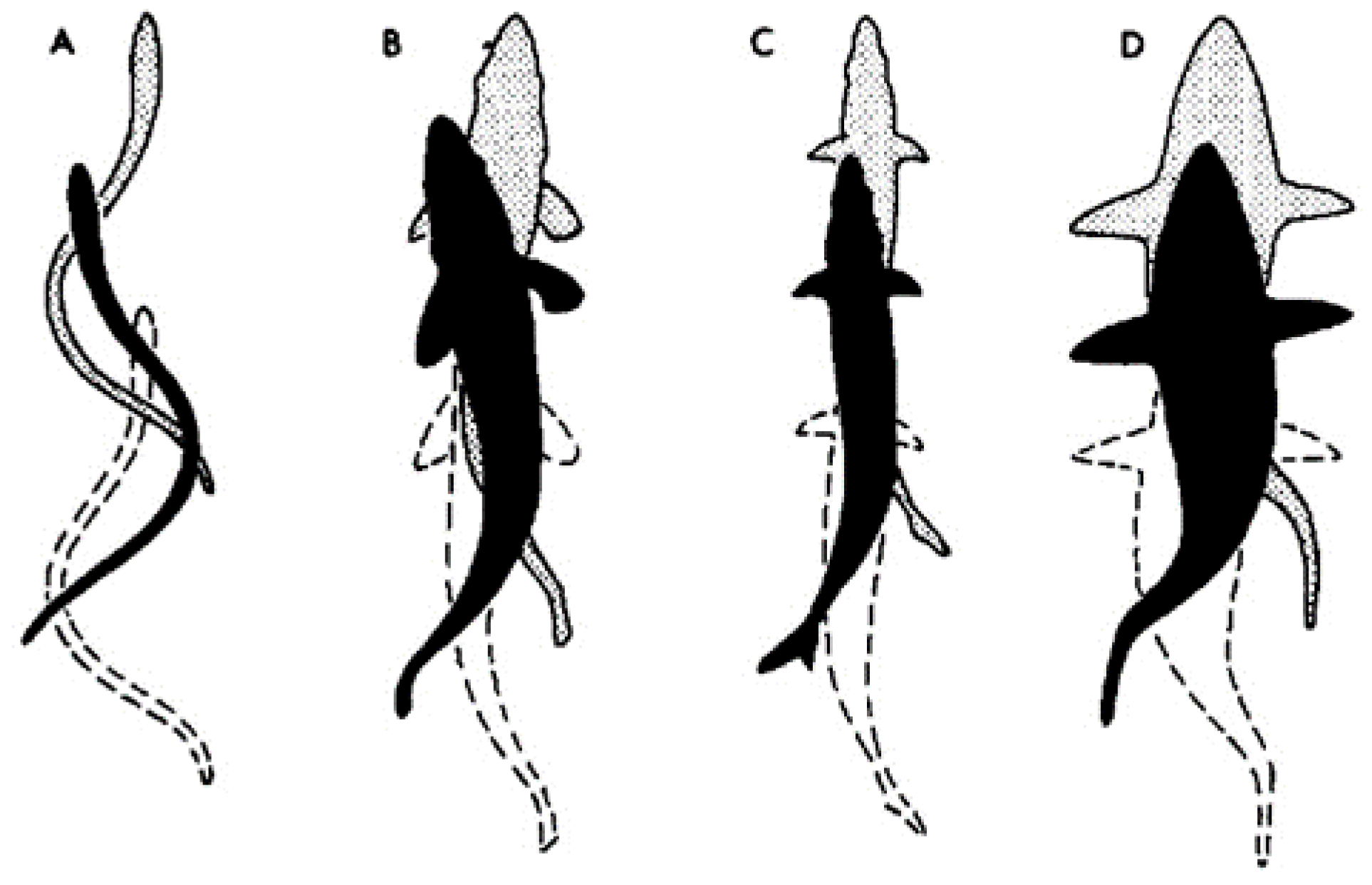
2.1. Swimming Styles

Undulatory and oscillatory swimming are two fundamental modes of aquatic locomotion, each characterized by unique propulsion methods and body kinetics (as shown in Figure 1). Undulatory swimmers, including eels and lampreys, propel themselves forward by creating sinuous, wave-like motions that travel along their bodies. This rhythmic flexion generates efficient thrust for propulsion. On the other hand, oscillatory swimmers like tuna and rays employ the back-and-forth movement of their caudal fins to generate thrust, often involving lifting and tilting motions. These distinct modes of swimming enable precise navigation in aquatic environments.

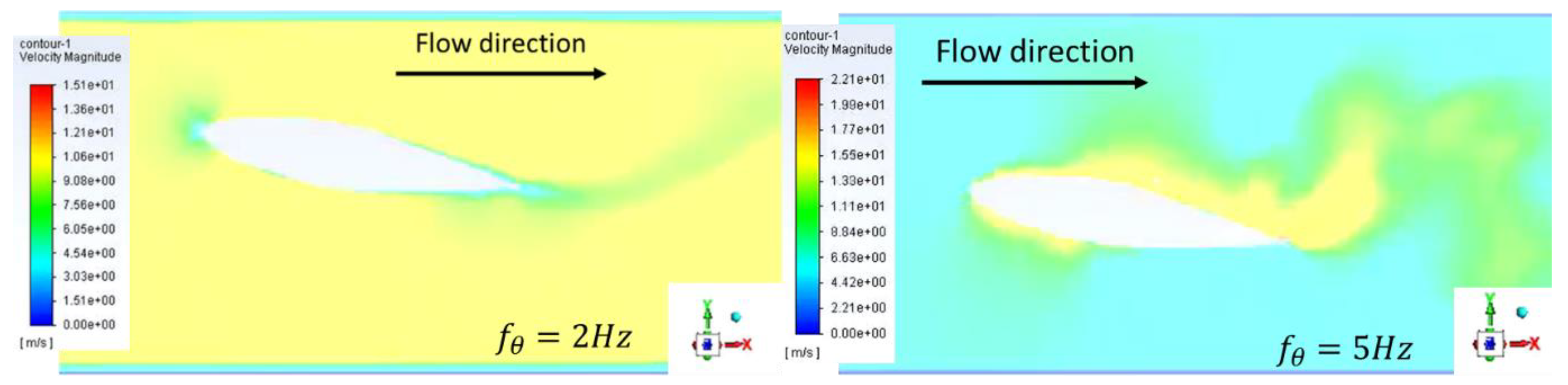
2.1.1. Oscillatory Motion

Efficient sustained cruise swimming in certain aquatic animals is characterized by a streamlined fusiform body shape, with the maximum depth around the midsection. This body structure aligns with their unique swimming motion and helps minimize recoil [11].

Some swimmers benefit from the cancellation of unsteady side forces and yawing moments due to the presence of at least one body-length wavelength (as shown in Figure 2). Others compensate for this lack by featuring a deep anterior body that narrows towards the posterior. They create thrust by tilting this force forward through fin movement perpendicular to the flow. Unlike propellers that rotate the wing around an axis, these swimmers oscillate their fins back and forth (as shown in Figure 3). This oscillation generates lateral forces that do not contribute to thrust and could induce swimming recoil. However, these side forces tend to cancel out over a single flapping cycle, and any remaining recoil is offset by other appendages [12,13].

To specify the motion of a dynamic zone in Ansys Fluent, we use DEFINE_CG_MOTION. This requires providing linear and angular velocities at each time step, which Ansys Fluent uses to update node positions. It is essential to remember that UDFs created with DEFINE_CG_MOTION can only run as compiled UDFs.

$$\dot{x}=\frac{2x}{2f_{\theta }\times \tan \theta }$$

(1)

$$\dot{y}=-y\times f_{\theta }\times \sin (f_{\theta }\times t)$$

(2)

$$\dot{\omega }=-\omega \times f_{\theta }\times \cos (f_{\theta }\times t)$$

(3)

where

$\dot{x}, x$ is the position and velocity in the x direction (m/s, m);

$\dot{y}, y$ is the position and velocity in the y direction (m/s, m);

$\dot{\omega }, \omega$ is the angular amplitude and angular velocity (rad/s, rad);

$f_{\theta }$ is the flapping frequency (Hz);

$\theta$ calculates the maximum angular displacement in radians.

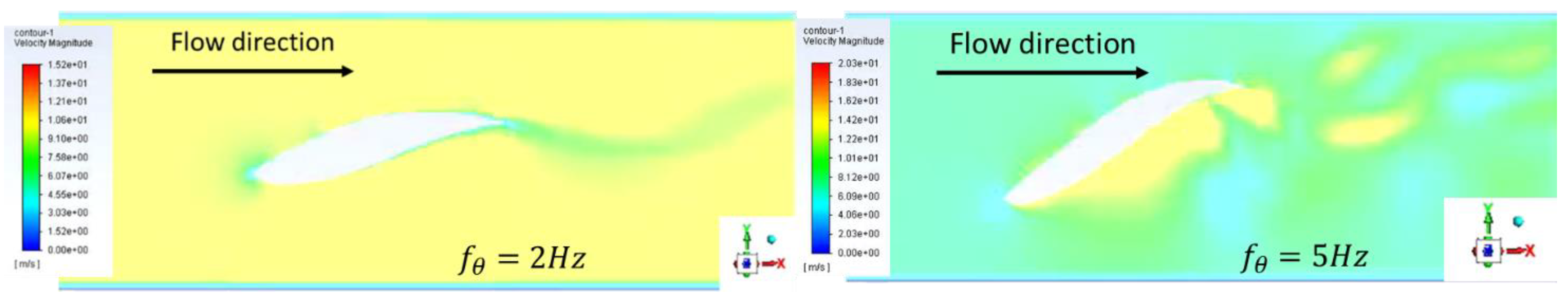
2.1.2. Undulatory Motion

To estimate thrust in slender aquatic animals like snakes, eels, and marine worms, a method was developed (as shown in Figure 4). It involves analyzing the equilibrium of a flexible cylinder in water with constant-amplitude bending waves traveling down it at a fixed speed. This approach, known as the ‘resistive model’ of thrust production, calculates total thrust by integrating segment contributions along the body length.

This approach, while valuable, has limitations. It assumes small-amplitude bending waves, quasi-steady resistive forces for each segment, and drag coefficients based on experiments with steady cylinders. For high Reynolds number flows with significant accelerations and added mass effects, slender body theory-based approaches have largely replaced resistive models. Nevertheless, the resistive model is still useful for low Reynolds number applications, adapting to different cross-sections, locomotion profiles, and a wide range of Reynolds numbers [15].

The wave begins small at the head and grows as it moves along the body. A more flexible tail with increased wave amplitude boosts tail inclination and improves thrust [16]. By default, Ansys Fluent updates node positions on a dynamic zone using the solid-body motion equation, resulting in no relative motion among the nodes. If individual control over node motion is needed, the DEFINE_GRID_MOTION UDF (User-Defined Function) is an option. This UDF allows for updating node positions, potentially incorporating deflections caused by fluid–structure interaction. However, UDFs created with DEFINE_GRID_MOTION can only be used in compiled UDF form [17].

$$y_n\left(t\right)=\sum _{n=1}^{\mathrm{\infty }}{y}_i\sin \left(2\pi f_{\theta }\times t_n\right)-2\pi \times \frac{x\times k}{l}$$

(4)

$$y_{n-1}\left(t\right)=\sum _{n=1}^{\mathrm{\infty }}{y}_i\sin \left(2\pi f_{\theta }\times t_{n-1}\right)-2\pi \times \frac{x\times k}{l}$$

(5)

where

$y_n, y_{n-1}$ is the amplitude, y, and depends on the time step;

$t_n,t_{n-1}$ is the time step;

$x$ is the x coordinate that determines y in the time step;

$f_{\theta }, k$ is the flapping frequency and wavenumber;

$l$ is the characteristic linear dimension.

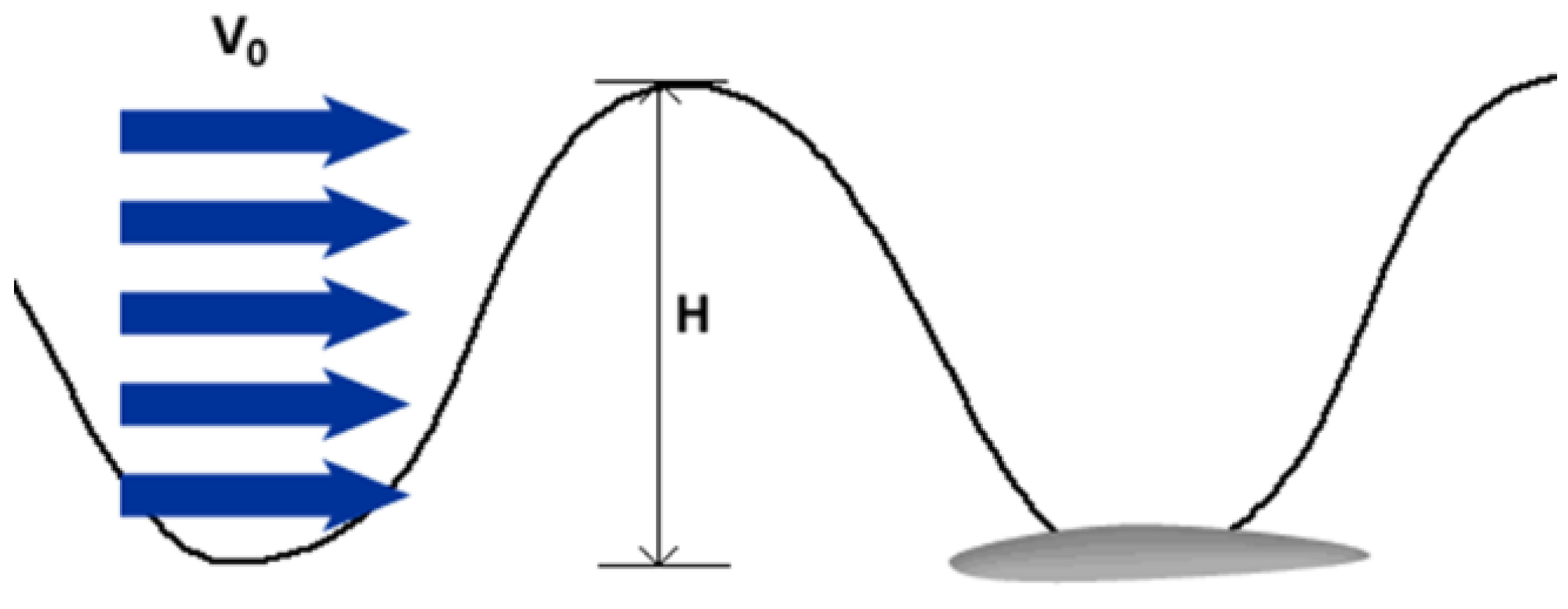
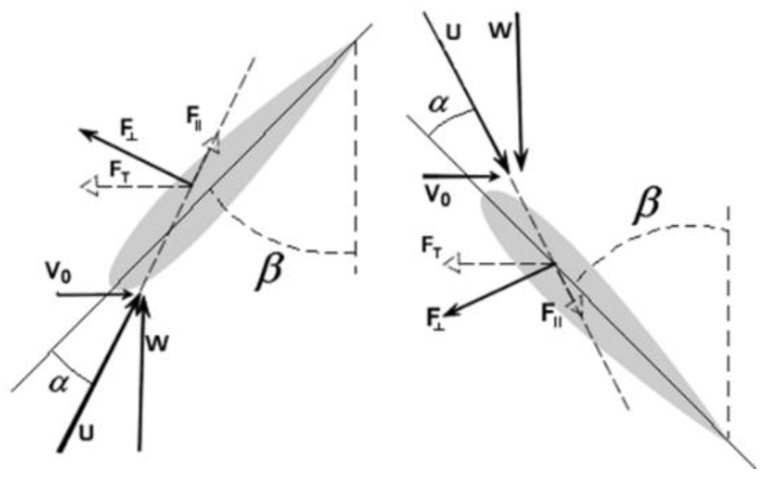
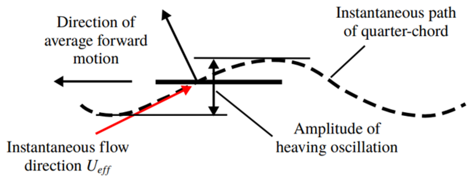
2.2. Mathematical Modeling

To study single-phase flow around robotic fish, three-dimensional, steady-state, incompressible, isothermal, and turbulent flow is considered. The mass conservation equation is as follows:

$$\frac{\partial \mathsf{\rho }}{\partial \mathrm{t}}+\nabla ·\left(\mathsf{\rho }\mathrm{U}\right)=0$$

(6)

The momentum conservation equation is as follows:

$$\frac{\partial \left(\rho U\right)}{\partial t}+\nabla ·\left(\rho U·U\right)-\nabla ·\left({\nu }_{eff}\nabla U\right)=-\nabla p^{\prime }+\nabla ·{\left({\nu }_{eff}\nabla U\right)}^T+\rho g$$

(7)

where $p^{\prime }$ is the corrected pressure, $g$ is the local gravity acceleration vector (adopted value $9.81 \mathrm{m}/{\mathrm{s}}^2$), and ${\nu }_{eff}$ is the effective viscosity, calculated as follows:

$${\nu }_{eff}=\nu +{\nu }_t$$

(8)

where

${\nu }_{eff}$ is the effective viscosity;

$\nu$ is the kinematic viscosity;

${\nu }_t$ is the turbulence viscosity.

Incorporating turbulence model equations is essential for capturing the turbulent phenomenon within the flow. Turbulence encompasses dynamic fluctuations in both time and space within the velocity and pressure fields. This intricate process can profoundly influence the flow’s behavior. Turbulence arises when the inertial forces exerted on the fluid outweigh the viscous forces, typically manifesting in flows with high Reynolds numbers. Additionally, turbulence can be induced by surface roughness, giving rise to secondary flow patterns [18]. Mesh for mathematical modeling is shown in Figure 5.

The exact $k-\epsilon$ equations contain many unknown and unmeasurable terms. For a much more practical approach, the standard $k-\epsilon$ turbulence model is used, which is based on our best understanding of the relevant processes, thus minimizing unknowns and presenting a set of equations which can be applied to a large number of turbulent applications. For turbulent kinetic energy, $k$,

$$\frac{\partial \left(\rho k\right)}{\partial t}+\frac{\partial \left(\rho k{u}_i\right)}{\partial x_i}=\frac{\partial }{\partial x_i}\left[\frac{u_i}{{\sigma }_k}\frac{\partial k}{\partial x_j}\right]+2{\mu }_i{E}_{ij}{E}_{ij}-\rho \epsilon$$

(9)

For dissipation, $\epsilon$,

$$\frac{\partial \left(\rho \epsilon \right)}{\partial t}+\frac{\partial \left(\rho \epsilon u_i\right)}{\partial x_i}=\frac{\partial }{\partial x_j}\left[\frac{u_i}{{\sigma }_{\epsilon }}\frac{\partial \epsilon }{\partial x_j}\right]+C_{1\epsilon }\frac{\epsilon }{k}2{\mu }_i{E}_{ij}{E}_{ij}-C_{2\epsilon }\rho \frac{{\epsilon }^2}{k}$$

(10)

The rate of change in $k$ or $\epsilon$ in time + the transport of $k$ or $\epsilon$ by advection = the transport of $k$ or $\epsilon$ by diffusion + the rate of production of $k$ or $\epsilon$—the rate of destruction of $k$ or $\epsilon$ [19], where

$u_i$ is the velocity component in corresponding direction;

$E_{ij}$ is the component of rate of deformation;

${\mu }_i=\rho C_{\mu }\frac{k^2}{\epsilon }$ is the Eddy viscosity.

The equations also consist of some adjustable constants, ${\sigma }_k=1.00, {\sigma }_{\epsilon }=1.30, C_{1\epsilon }=1.44, C_{2\epsilon }=1.92, \mathrm{a}\mathrm{n}\mathrm{d} C_{\mu }=0.09$. The values of these constants have been arrived at by numerous iterations of data fitting for a wide range of turbulent flows.

Viscosity affects fluid flow near surfaces, reducing momentum within the boundary layer and influencing overall behavior. This interaction requires analyzing viscosity’s retarding effect and the associated pressure distribution to determine the drag coefficient. Drag on a submerged body combines frictional drag, from surface shear stress, and pressure drag, related to flow pressure variations and wake formation. A dimensionless drag coefficient quantifies these interactions. The total drag coefficient is calculated by the following [20]:

$$C_D=C_F+C_P=\frac{0.075}{{\left({\log }_{10}Re-2\right)}^2}+\frac{F_P}{0.5\rho U^2{S}_0}$$

(11)

where $C_D$ is the total drag coefficient, $C_F$ is the friction drag coefficient, $C_P$ is the pressure drag coefficient, $F_P$ is the pressure drag force, $U$ is the free stream parallel fluid velocity, $S_0$ the wetted surface area at rest, and $F_D$ is the drag force [21].

The Reynolds number is the ratio of inertial forces to viscous forces within a fluid subjected to relative internal movement due to different fluid velocities. A region where these forces change behavior is known as a boundary layer. This relative movement generates fluid friction, a factor in developing turbulent flow. Counteracting this effect is the fluid’s viscosity, which tends to inhibit turbulence. The Reynolds number quantifies the relative importance of these two types of forces for given flow conditions and is a guide to when turbulent flow will occur in a particular situation:

$$Re=\frac{UL}{\upsilon }$$

(12)

where $U$ is the flow speed (m/s), $L$ is a characteristic length (m), and $\upsilon$ is the kinematic viscosity of the fluid (m²/s).

In dimensional analysis, the Strouhal number is a dimensionless number describing oscillating flow mechanisms. The Strouhal number is an integral part of the fundamentals of fluid mechanics. The Strouhal number is often given as

$$St=\frac{fL}{U}$$

(13)

where $f$ is the frequency of vortex shedding. The Strouhal number represents the ratio of inertial forces due to the local acceleration of the flow to the inertial forces due to the convective acceleration. Depending on the time scale of the problem, this ratio may be of order unity, and, therefore, its importance is not obvious [22].

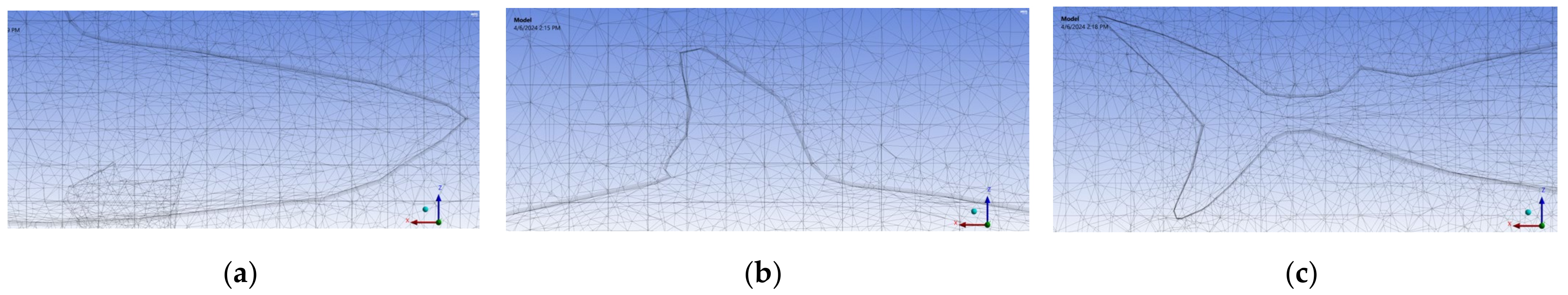
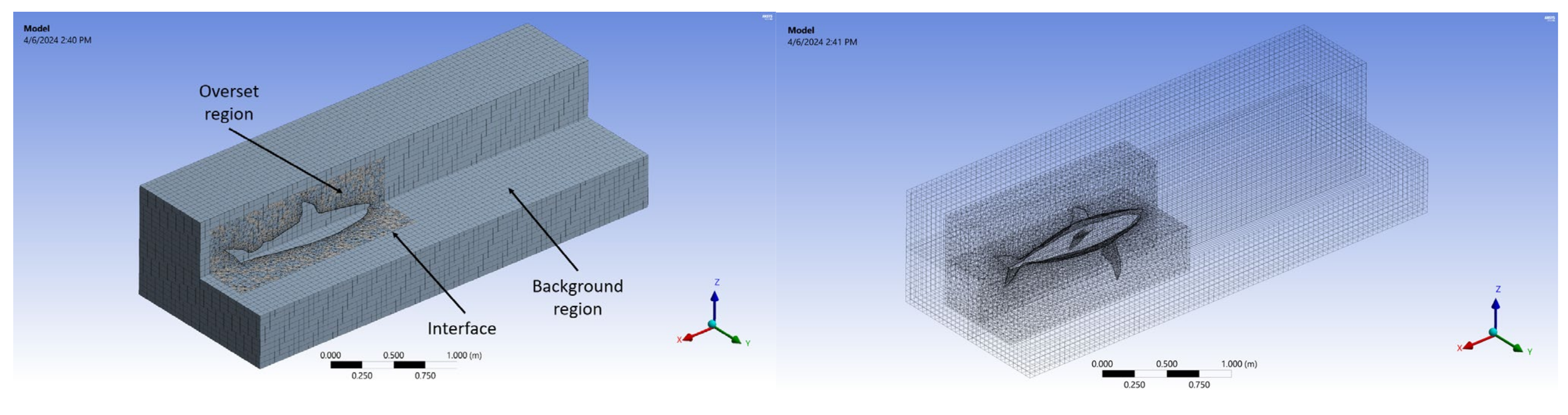
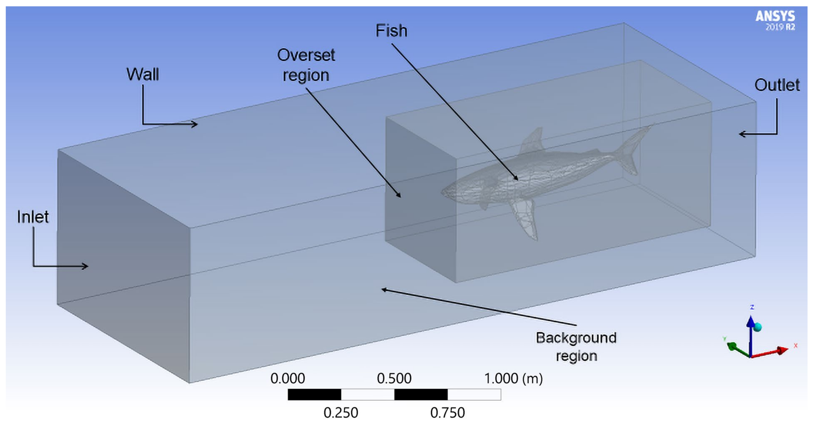
2.3. The Numerical Meshes and Boundary Conditions

The use of an overset mesh, also known as “chimera” or “overlapping” mesh, can streamline and expedite simulations involving moving components. Complex fluid flow simulations often encounter challenges when representing certain geometries with a single contiguous mesh. In such cases, different mesh types may be best-suited for distinct geometric features, making the preparation of a unified mesh time-consuming and intricate. This can lead to the creation of large poorly structured meshes that demand excessive solving time and compromise accuracy [19].

Ansys Fluent offers support for overset mesh, which proves valuable in optimizing simulations encompassing various aspects, including structured mesh around individual parts, part swapping, moving cell zones (eliminating the need for remeshing or smoothing), and design exploration studies (as shown in Figure 6). Overset mesh is particularly advantageous when dealing with significant relative motion between components. In comparison to remeshing, it provides enhanced control over local mesh characteristics as the geometry moves within the domain, as individual mesh zones do not need to deform to accommodate moving geometry. When applied appropriately, overset mesh can facilitate the optimization of local cell types and quality, reduce cell count (thus decreasing computation time), and simplify model setup. This technology, complemented by other robust mesh-related features in Ansys Fluent, forms a comprehensive toolkit for simulating fluid dynamics in the presence of intricate moving geometries [16].

Overset mesh limitations include several constraints to consider. Firstly, the overset interface cannot encompass solid cell zones. Secondly, component meshes cannot establish connections with a non-conformal interface. Additionally, background meshes should not feature non-conformal interfaces between them, and component zones are restricted from having periodic boundaries. It is worth noting that for all overset mesh problems, it is recommended to utilize double precision. These limitations underscore the importance of careful planning and adherence to guidelines when working with overset mesh techniques in simulations. The boundary conditions are shown in Figure 7 and

Table 1. Parameter conditions used in the simulations.

Properties	Condition	Value
Inlet	Prescribed velocity	1–4 m/s
Outlet	Prescribed pressure	Gauge pressure
Fish surface	Prescribed velocity
Wall	No slip and smooth wall
Overset region	Inner interior
Background region	Outer interior
Density of water	-	$999.7 \mathrm{k}\mathrm{g}/{\mathrm{m}}^3$
Kinematic viscosity	-	$1.3084\times {10}^{-6} {\mathrm{m}}^2/\mathrm{s}$

.

This model was calibrated using numerical simulations in conjunction with the least-square error technique. All simulations were performed using the commercial software Ansys Fluent 19.0, which employs the finite volume method based on finite elements to address the research problem.

3. Results and Discussion

3.1. Robotic Fish with Different Base Dimension

The 3D model is meticulously crafted and edited with the assistance of Rhino 6 software (as shown in Figure 8). This software not only facilitates the construction of intricate models but also offers convenient accessibility to the body plan, making it exceptionally well-suited for manufacturing applications.

The entire calculation is performed with dimensionless parameters.

Implementation of the dimensionless model is shown in Figure 9 and Figure 10. Expressing the body’s meridian section equation in coordinates ($X, Y$) using a polynomial for the sectional–area curve [23] is shown as

$$\pi Y^2=A_{1}X+A_2{X}^2+\dots +A_n{X}^n$$

(14)

The function f($x$) is of degree six, while the function f($y$) is of degree two:

$$y^2=a_{1}x+a_2{x}^2+\dots +a_n{x}^n$$

(15)

The dimensionless combinations of the primary geometric quantities are as follows:

$$x=\frac{X}{L},y=\frac{Y}{d};m=\frac{x_m}{L}; r_o=\frac{R_{o}L}{d^2}; r_t=\frac{R_{t}L}{d^2}$$

(16)

Figure 9. Principal dimensions of a body of revolution.

Figure 9. Principal dimensions of a body of revolution.

Figure 10. Nondimensional representation of a sectional–area curve.

Figure 10. Nondimensional representation of a sectional–area curve.

Table 2. Fish parameters used in the simulations.

Notation	Unit	Range
$L$	m	0.3–1.2	The length
$d$	m	0.3	The maximum diameter
$x$	(Dimensionless)	0–1	The axial
$y$	(Dimensionless)	0–0.1	The radius
$m$	(Dimensionless)	0.4	The distance of the maximum section from the nose
$r_o$	(Dimensionless)	0.1	The radius of curvature at the nose
$r_t$	(Dimensionless)	0.1	The radius of curvature at the tail
$a_n$	(Dimensionless)		The shape coefficients

is used to explain the notation in Equations (14). The model utilized in this research study is derived from approximate specifications representing an adult shark. It is important to note that this model is primarily designed for conducting computational fluid dynamic (CFD) simulations rather than resembling a robotic fish. Consequently, various details typically associated with a robotic fish, such as joints, connections, and openings, have intentionally been omitted from the design. This streamlined and simplified approach ensures that the model serves its primary purpose of facilitating CFD simulations effectively, allowing for a focused and comprehensive analysis of fluid dynamics and related phenomena without unnecessary complexities (as shown in Figure 11).

To perform this simulation, the initial step involves creating a 3D model of the object or structure for which drag force calculations are required. This model should include all relevant surfaces and boundary conditions necessary for the simulation. Once the model is prepared, Ansys Fluent is used to set up the simulation project. This involves specifying the flow conditions, initial pressures, and boundary conditions. Turbulence model k-epsilon is chosen to accurately capture turbulent effects. Within the simulation setup, the drag force calculation feature is enabled. Once all parameters are configured, the simulation is executed. Ansys Fluent utilizes the provided information about the flow and object geometry to calculate the drag force based on the Navier–Stokes equations and relevant experimental or computational data. Upon completion of the simulation, the results are available for analysis within Ansys Fluent, displaying the magnitude and direction of the calculated drag force. These results are invaluable for optimizing designs, assessing performance, and making informed decisions in engineering and design processes.

The flow velocity across the range of 1 to 4 m/s exhibits an interesting trend in the context of drag coefficient calculations. While one might intuitively expect an increase in drag coefficient with higher flow velocities due to increased fluid resistance, the observed results from both theoretical and numerical methods are different. The average theoretical drag coefficient recorded in these conditions is approximately 0.256. This finding suggests that the fish model under consideration may exhibit unique hydrodynamics, leading to a nonlinear relationship between velocity and drag (as shown in

Table 3. Comparison between theoretical and numerical results of the drag coefficients for flow.

U (m/s)	$\mathit{R}\mathit{e}\times {10}^6$ (−)	Theoretical	Numerical	Difference between Numerical and Theoretical (%) $\frac{\left|{\mathit{C}}_{\mathit{D}}\mathbf{n}\mathbf{u}\mathbf{m}\mathbf{e}\mathbf{r}\mathbf{i}\mathbf{c}\mathbf{a}\mathbf{l}-{\mathit{C}}_{\mathit{D}}\mathbf{t}\mathbf{h}\mathbf{e}\mathbf{o}\mathbf{r}\mathbf{e}\mathbf{t}\mathbf{i}\mathbf{c}\mathbf{a}\mathbf{l}\right|}{{\mathit{C}}_{\mathit{D}}\mathbf{t}\mathbf{h}\mathbf{e}\mathbf{o}\mathbf{r}\mathbf{e}\mathbf{t}\mathbf{i}\mathbf{c}\mathbf{a}\mathbf{l}}\times 100\mathit{\%}$
1.0	1.146	0.264	0.290	9.930
1.5	1.720	0.260	0.282	8.297
2.0	2.293	0.257	0.277	7.607
2.5	2.866	0.255	0.274	7.097
3.0	3.439	0.254	0.271	6.794
3.6	4.127	0.251	0.268	6.544
4.0	4.586	0.250	0.266	6.345

). Conversely, when employing numerical methods to calculate the drag coefficient, the trend still shows a decrease in this coefficient as the flow velocity increases, although the decrease is not substantial. The average simulation-based drag coefficient under these conditions is approximately 0.275. This observation implies that the simulation accounts for certain complexities or factors that influence drag differently than what is typically captured by theoretical measurements.

Upon analyzing the outcomes, it becomes evident that the disparities between the predicted and theoretical drag coefficients are relatively minor. Specifically, the maximum difference stands at 9.93%, while the average difference is a mere 7.516% (as shown in Figure 12). These variations can be ascribed to a combination of factors, including theoretical inaccuracies, numerical approximations, and the slight distinctions between the hull geometry employed in computational simulations and that employed in the theoretical setup. The narrow discrepancies observed across the results serve as a validation of the methodology adopted in this study, affirming its capability to accurately depict the underlying physical phenomenon under investigation.

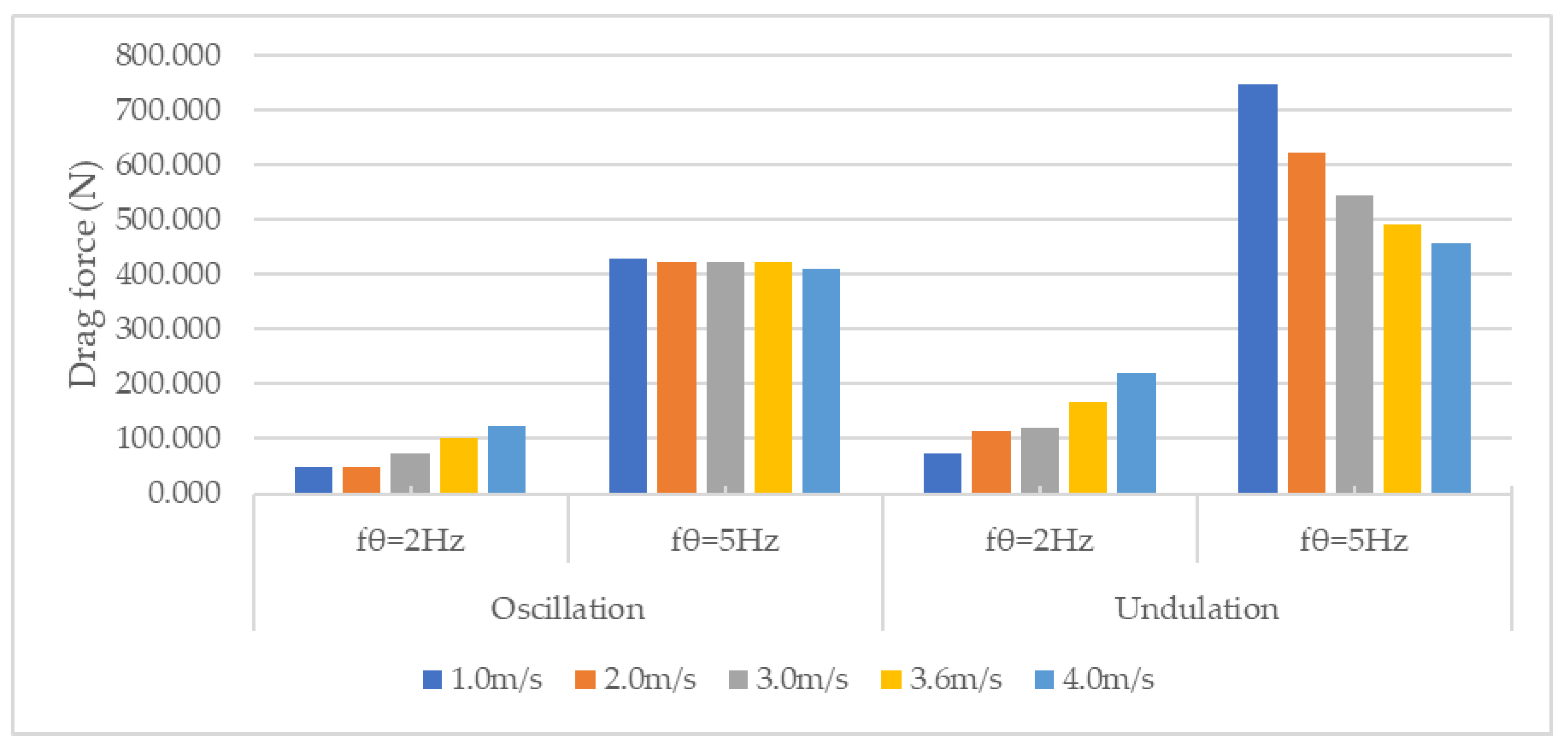
3.2. Robotic Fish with Oscillatory and Undulatory Motion

The first simulation involves oscillation in two primary directions: investigating variations in flapping frequency and its interaction with the flow. During each up or down cycle of the model, resistance is generated across the entire wetted surface, resulting in rearward thrust opposing the direction of motion. It is crucial to emphasize that the drag coefficient of a particular foil depends not only on its profile shape but also on its Reynolds number. Thus, maximizing thrust and efficiency at a specific Reynolds number presents an optimization challenge, requiring the identification of the model shape with the lowest drag coefficient for a given motion profile (as shown in Figure 13).

The dorsal fin in ray-finned fish generates significant lateral momentum during locomotion, resulting in roll and yaw torques. To achieve stable swimming, other fins must counterbalance these torques. The tail fin may offset roll torques, and coordination between the tail and pectoral fins helps correct yaw torques. Theoretical research highlights the existence of a multifaceted force equilibrium among all fins, the body, and the tail, even during consistent swimming. This challenges the conventional classification of locomotion as either BCF (body-caudal fin) or MPF (median-paired fin), as median fins actively contribute to body stability (as shown in Figure 14).

To comprehend this force equilibrium, data on buoyancy, body shape, and fin forces are crucial. Fish frequently maintain a positive angle of attack to their bodies, impacting lift forces due to body airflow. The three-dimensional flow dynamics around the body and tail introduce further complexity. Vortex wake patterns generated by different fins interact, creating a dynamic hydrodynamic environment. Comprehensive theoretical investigation is essential to fully grasp these interactions, underscoring the significance of three-dimensional effects in understanding fish undulatory hydrodynamics.

At a flapping frequency of 2 Hz, it is observed that both types of motion experience a reduction in their respective drag coefficients, while the overall drag forces they encounter increase. Upon closer examination of each specific motion, it becomes apparent that the undulatory motion exhibits a higher drag coefficient when compared to the oscillatory motion. Conversely, the oscillatory motion demonstrates a lower drag force in comparison to the undulatory motion. These findings suggest that the dynamics of these two distinct types of motion play a crucial role in shaping their drag characteristics, with undulatory motion displaying a more pronounced resistance to flow and oscillatory motion exhibiting a relatively lower drag force (as shown in Figure 15 and

Table 4. The drag coefficient and drag force for each type of motion depending on the flow velocity.

Flow Velocity (m/s)	$\mathbf{Flapping} \mathbf{Frequency} {\mathit{f}}_{\mathit{\theta }}=2 \mathbf{H}\mathbf{z}$					$\mathbf{Flapping} \mathbf{Frequency} {\mathit{f}}_{\mathit{\theta }}=5 \mathbf{H}\mathbf{z}$
	St	Oscillation		Undulation		St	Oscillation		Undulation
		${\mathit{C}}_{\mathit{D}}$	${\mathit{F}}_{\mathit{D}}$ (N)	${\mathit{C}}_{\mathit{D}}$	${\mathit{F}}_{\mathit{D}}$ (N)		${\mathit{C}}_{\mathit{D}}$	${\mathit{F}}_{\mathit{D}}$ (N)	${\mathit{C}}_{\mathit{D}}$	${\mathit{F}}_{\mathit{D}}$
1.0	0.300	1.812	47.931	4.497	73.343	0.750	16.228	429.269	28.196	745.845
2.0	0.150	0.450	47.635	0.693	112.677	0.375	3.993	422.462	5.874	621.566
3.0	0.100	0.314	74.845	0.516	118.954	0.250	1.830	422.292	2.283	543.528
3.6	0.083	0.296	101.434	0.486	166.652	0.208	1.232	422.245	1.430	490.055
4.0	0.075	0.291	123.065	0.473	218.566	0.188	0.969	409.942	1.077	455.868

).

In contrast to the 2 Hz flapping frequency, there are distinct results observed at the 5 Hz flapping frequency. At 5 Hz, the drag coefficient is significantly higher compared to 2 Hz, although it still exhibits a decreasing trend. The drag force at 5 Hz is also greater than at 2 Hz, but there is a notable difference: it decreases as the flow velocity increases. When examining each motion separately, the undulatory motion still maintains a higher drag coefficient than the oscillatory motion. However, as velocities get higher, the drag force decreases and now becomes closer between the two types of motion.

4. Conclusions

This research uniquely concentrates on a detailed examination of fish motion, particularly highlighting the intricacies of undulating and oscillatory movements, distinguishing itself from current studies. The emphasis shifts towards utilizing kinematic equations of motion control for fluid dynamic calculations. The design, created using Rhino 6 software, incorporates precise fluid resistance computations via Ansys Fluent 19, investigating flow velocities spanning from 1 to 4 m/s.

As flow velocity linearly increases, the drag force exhibits an inverse variation in tail flap frequency between oscillation and undulation. Using this information, optimization of the motion control equation is necessary for attaining maximum thrust under various tail flapping frequencies causing a resistance to surge. Remarkably, at high tail flapping frequencies, a decreasing trend in drag force is observed (746 N at 1 m/s and 456 N at 4 m/s). The integration of kinematic equations of motion control has facilitated the discovery of this intriguing phenomenon. This research has contributed to analyzing the development of fish shape and motion control to generate thrust under various flapping frequencies from 2 Hz to 5 Hz and under various flow velocities from 1 m/s to 4 m/s.

References

1. Jackson, S. Argo: The first ship? Rhein. Mus. Philol. 1997, 140, 249–257. [Google Scholar]
2. Yang, B.; Liu, Y.; Liao, J. Manned Submersibles—Deep-sea Scientific Research and Exploitation of Marine Resources. Bull. Chin. Acad. Sci. 2021, 36, 622–631. [Google Scholar]
3. Williams, S.B.; Newman, P.; Rosenblatt, J.; Dissanayake, G.; Durrant-Whyte, H. Autonomous underwater navigation and control. Robotica 2001, 19, 481–496. [Google Scholar] [CrossRef]
4. Kramer, B. Electroreception and Communication in Fishes; Gustav Fischer: Stuttgart, Germany, 1996; Volume 42. [Google Scholar]
5. Soomro, A.M.; Memon, F.H.; Lee, J.W.; Ahmed, F.; Kim, K.H.; Kim, Y.S.; Choi, K.H. Fully 3D printed multi-material soft bio-inspired frog for underwater synchronous swimming. Int. J. Mech. Sci. 2021, 210, 106725. [Google Scholar] [CrossRef]
6. Cohen, R.C.Z.; Cleary, P.W. Computational Studies of the Locomotion of Dolphins and Sharks Using Smoothed Particle Hydrodynamics. In Proceedings of the 6th World Congress of Biomechanics (WCB 2010), Singapore, 1–6 August 2010. [Google Scholar]
7. Sun, K.; Cui, W.; Chen, C. Review of Underwater Sensing Technologies and Applications. Sensors 2021, 21, 7849. [Google Scholar] [CrossRef] [PubMed]
8. Alexander, J. Smits, Undulatory and oscillatory swimming. J. Fluid Mech. 2019, 874, P1. [Google Scholar] [CrossRef]
9. Alam, M.I.; Pant, R.S. Estimation of Volumetric Drag Coefficient of Two-Dimensional Body of Revolution. J. Aircr. 2019, 56, 5. [Google Scholar] [CrossRef]
10. Nesteruk, I.; Passoni, G.; Redaelli, A. Shape of Aquatic Animals and Their Swimming Efficiency. J. Mar. Biol. 2014, 2014, 470715. [Google Scholar] [CrossRef]
11. Muratoglu, A.; Yuce, M.I.; Eşit, M. Foil Generation Inspiring from Nature. In Proceedings of the International Conference on Natural Science and Engineering, ICNASE’16, Kilis, Turkey, 19–20 March 2016. [Google Scholar]
12. Lighthill, M.J. Note on the swimming of slender fish. J. Fluid Mech. 1960, 9, 305–317. [Google Scholar] [CrossRef]
13. ISO 9001:2008; ANSYS FLUENT 12.0 UDF Manual. ANSYS, Inc.: Canonsburg, PA, USA, 2009.
14. Krueger, P.S. A Brief Introduction to Mechanical and Biological Propulsion. Available online: https://s2.smu.edu/propulsion/Pages/navigation.htm (accessed on 10 November 2023).
15. Lauder, G.V.; Tytell, E.D. Hydrodynamics of Undulatory Propulsion, Fish Biomechanics. Fish Physiol. 2005, 23, 425–468. [Google Scholar]
16. Li, N.; Liu, H.; Su, Y. Numerical study on the hydrodynamics of thunniform bio-inspired swimming under self-propulsion. PLoS ONE 2017, 12, e0174740. [Google Scholar] [CrossRef] [PubMed]
17. Tay, C.M.J.; Khoo, B.C.; Chew, Y.T. Mechanics of drag reduction by shallow dimples in channel flow. Phys. Fluids 2015, 27, 035109. [Google Scholar] [CrossRef]
18. Neveln, I.D.; Bale, R.; Bhalla, A.P.S.; Curet, O.M.; Patankar, N.A.; MacIver, M.A. Undulating fins produce off-axis thrust and flow structures. J. Exp. Biol. 2014, 217, 201–213. [Google Scholar] [CrossRef]
19. Nesteruk, I. Drag Drop on High-Speed Supercavitating Vehicles and Supersonic Submarines. Appl. Hydromechnics 2015, 17, 52–57. [Google Scholar]
20. Wu, T.Y. Fish Swimming and Bird/Insect Flight. Annu. Rev. Fluid Mech. 2011, 43, 25–58. [Google Scholar] [CrossRef]
21. 7.5-02-02-02; ITTC 1957 Recommended Procedures and Guidelines. ITTC: Zürich, Switzerland, 2011.
22. Journée, J.M.J.; Massie, W.W. Offshore Hydromechanics; Delft University of Technology: Delft, The Netherlands, 2001. [Google Scholar]
23. Landweber, L.; Gertler, M. Mathematical Formulation of Bodies of Revolution; DTMB-719; David Taylor Model Basin: Washington, DC, USA, 1950. [Google Scholar]
Figure 1. Gradation of swimming modes from (A) anguilliform, through (B) subcarangiform, to (C) carangiform, and (D) thunniform.
Applsci 14 03239 g001
Figure 2. Incident flow and flapping object interaction [14].
Applsci 14 03239 g002
Figure 3. Riding along with the fin as it moves down-up.
Applsci 14 03239 g003
Figure 4. Lift-based thrust generation.
Applsci 14 03239 g004
Figure 5. Details of mesh around the regions of head (a), dorsal fin, (b) and tail (c).
Applsci 14 03239 g005
Figure 6. Meshes created in the studied domain.
Applsci 14 03239 g006
Figure 7. Physical specifications of the domain with the boundary conditions.
Applsci 14 03239 g007
Figure 8. Shape of the fish.
Applsci 14 03239 g008
Figure 11. Velocity field around the fish.
Applsci 14 03239 g011
Figure 12. The comparison of the drag coefficients between the results of theoretical and numerical methods.
Applsci 14 03239 g012
Figure 13. The velocity field around the oscillatory motion of the fish.
Applsci 14 03239 g013
Figure 14. The velocity field around the undulatory motion of the fish.
Applsci 14 03239 g014
Figure 15. The comparison of the drag force between the results of oscillation and undulation.
Applsci 14 03239 g015