Entropy Wavelet-Based Method to Increase Efficiency in Highway Bridge Damage Identification

Abstract

Highway bridges are crucial civil constructions for the transport infrastructure, which require proper attention from the corresponding institutions of each country and constant financing for their adequate maintenance; this is important because different types of damage can be generated within these structures, caused by natural disasters, among other sources, and the heavy loads they transport every day. Therefore, the development of simple, efficient, and low-cost methods is of vital importance, allowing us to identify damage in a timely manner and avoid bridges collapsing. As reported in a previous work, the wavelet energy accumulation method (WEAM) and its corresponding application in the Rio Papaloapan Bridge (RPB) represented an important advance within the field. Despite identifying damage in bridges with precision and at a low cost, there are several aspects to improve in that method. Therefore, in this work, that method was improved, eliminating several steps, and meaningfully reducing the computational burden by implementing an algorithm based on the Shannon entropy, thus giving way to the new entropy wavelet-based method (EWM). This new method was applied directly with regard to the real-life RPB, in both its healthy and damaged conditions. Also, its corresponding numerical model based on the finite element method in its healthy condition and different damage scenarios were carried out. The results indicate that the new EWM retains the advantages of WEAM, and it allows for damage identification to be completed more efficiently, increasing the precision by approximately 0.11%, and significantly reducing the computing time required to obtain results by 5.67 times.

1. Introduction

Due to the accelerated population growth in recent decades, the construction of cities, towns, and related infrastructures is essential for the adequate interaction of social, well-being, political, and economic activities in every nation around the world [1,2,3]. One of the most critical and expensive infrastructures that allows communication between different regions are bridges, which tend to deteriorate and accumulate diverse types of damage, produced by different environmental and human factors [4,5,6]. Therefore, damage to bridges, as in any civil structure, is inherent; however, those constructions can provide many years of surface with adequate maintenance programs and appropriate damage identification processes [7,8,9]. Thus, a periodical monitoring of civil structures called structural health monitoring (SHM) is fundamental for preserving the service life of bridges, and avoiding tragic accidents resulting from damage not being detected in time [10,11].

The global monitoring of bridges offers vital information regarding the serviceability and general integrity of the bridges; however, ensuring safety and continuous service depends on the methodology applied to identify damage in all of the critical elements in a timely, accurate, and efficient manner, as well as on the capacity to monitor the damage propagation and the decisions made to correct the structural defects without significantly affecting the operation of these structures. Bridge diagnosis comprises two levels being included in a damage identification process: the detection and localization of damage. As its name indicates, the damage detection alerts us about the existence of damage in the inspected structure, while the damage localization determines the position of the defects on the structure [12]. Failure to detect damage to bridges in a timely manner can cause collapses with tragic consequences. In this regard, an example of this kind of accident happening in the current century is the Entre-os-Rios tragedy, which was a disaster that occurred on 4 March 2001 in Porto Portugal, where the fourth pillar of the Hintze Ribeiro Bridge, which connected the towns of Castelo de Paiva and Eja over the Duero River, had suffered damage that was not detected in time, causing the collapse of two sections of the road and the death of 59 people in vehicles [13].

Similar to the bridge collapse described above, many catastrophic accidents have occurred due to failures, deteriorations, or the accumulation of damage in different elements of bridges, causing the collapse of entire structures and therefore devastating human deaths and substantial economic losses [14,15,16,17]. Historically, the damage identification process has been performed to visually monitor the condition of bridges. However, some important limitations of this process are a lack of regular monitoring, inspection-dependent monitoring, a delay in defect detection, and an inability to determine damage growth stages [18]. As an alternative to visual monitoring, systems based on SHM are used. In a typical SHM of bridges, sensors are dispersed throughout the structure, and the collected data are used to analyze the condition of the bridge [19,20,21]. Different parameters can be used to evaluate structures using SHM systems, such as corrosion, cracking, displacement, fatigue, settlement, deformation, temperature, inclination, vibration, water level, etc. [22]. Therefore, it is of vital importance to develop and implement reliable and low-cost methods for the detection and location of non-visible damage in bridges. In recent years, to address the need to safeguard the structural integrity of bridges, SHM systems have been developed worldwide, and different analysis methods for the detection, location, and evaluation of damage in bridges are being investigated.

In recent decades, SHM techniques, based on the analysis and post-processing of the vibration responses of bridges, have become the most promising alternatives used to efficiently detect, locate, and evaluate the severity of damage in this type of civil structure, guaranteeing its integrity and predicting its useful life [23,24]. Thus, vibration-based methods for identifying damage in structures subjected to moving loads, such as bridges, can be broadly classified into parametric and non-parametric methods [25]. Parametric methods work with data in the modal domain [26,27,28,29,30,31]. On the other hand, non-parametric methods use data in the time or frequency domain; these include wavelet theory [32,33,34,35], empirical mode decomposition [36,37,38], time series analysis [39,40,41], multiple signal classification [42,43], entropy [44,45,46,47], neural networks [48,49,50], fractals [51,52], principal component analysis [53,54,55,56], etc.

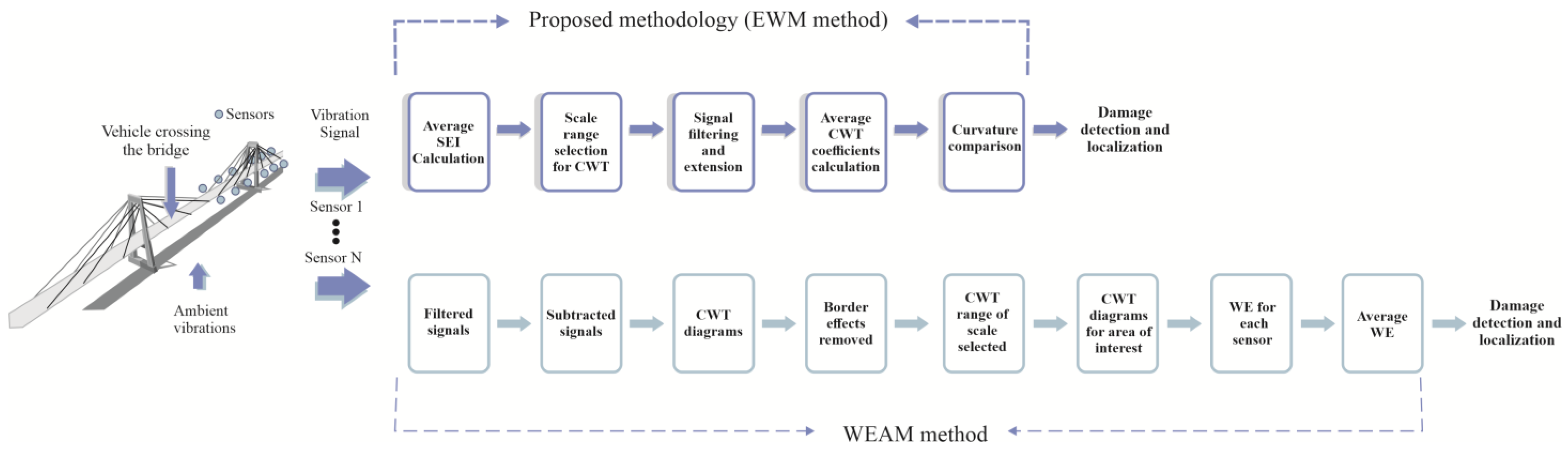
In particular, the wavelet energy accumulation method (WEAM) is a non-parametric method, previously developed in [1], with the objective of detecting and locating damage in vehicular bridges. This method overcomes the limitations of the parametric methods, and provides additional advantages from the previously developed non-parametric methods. Despite the advantages of WEAM, which include its ability to detect and locate diverse types of damage in bridges with high precision, in different locations, and of various severities via the use of a few sensors distributed on the bridge deck, its main disadvantages are that it involves a significant number of stages, as well as the requirement of a high computing time.

According to the aforementioned issues, in this article, a new method, called the entropy wavelet-based method (EWM), is presented, which eliminates the drawbacks of the WEAM via the implementation of an algorithm based on the Shannon entropy [57]. This method avoids the need of obtaining three-dimensional colored CWT (continuous wavelet transform) diagrams with very good resolutions, a very wide initial scale range, and the appropriate choice of the color map to begin investigating whether there has been damage caused to the analyzed bridge via the use of monitoring data, as well as in which area of those diagrams the damage identification is easier, which again requires a significant computing time. With the entropy-based algorithm that is developed and implemented in this study, it is possible to know the most convenient specific scale value or scale range in a very timely manner, allowing for the identification of damage without a loss of precision in the damage location, thus saving a significant amount of computational time; this will be of great help for practical systematic applications on the bridges of the Federal Highway Network of a specific country.

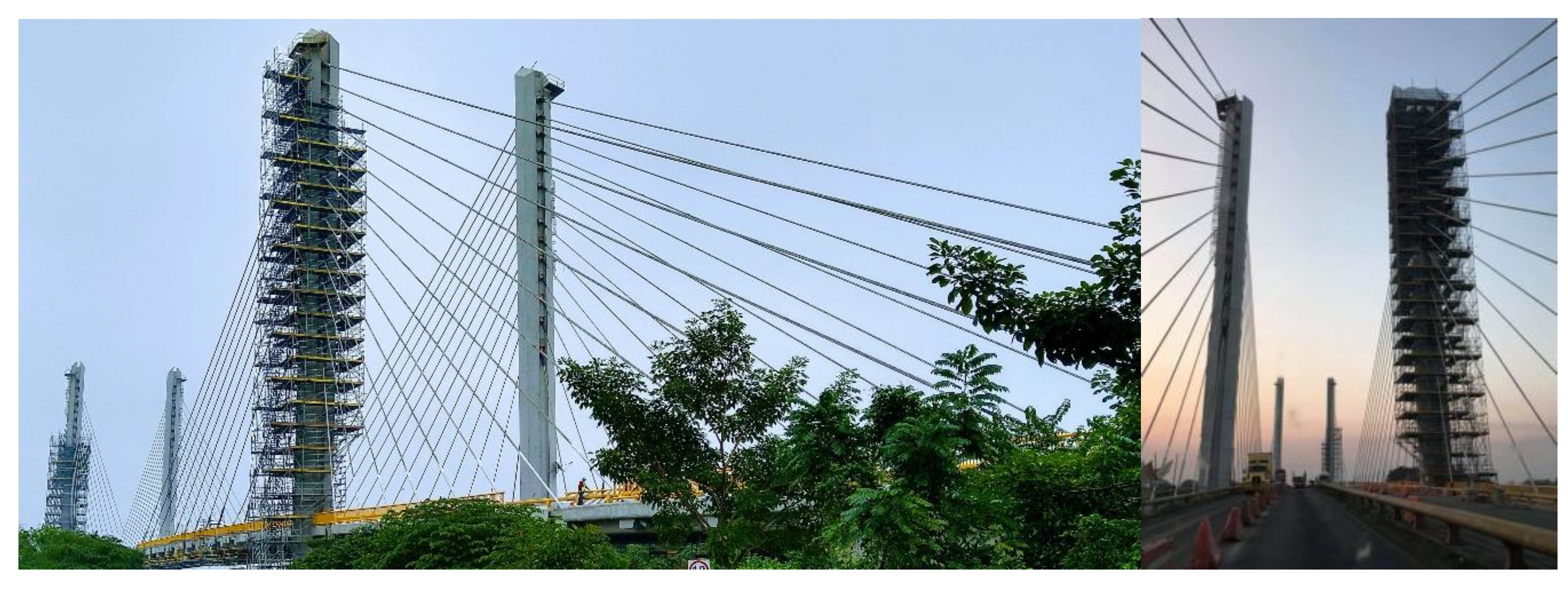
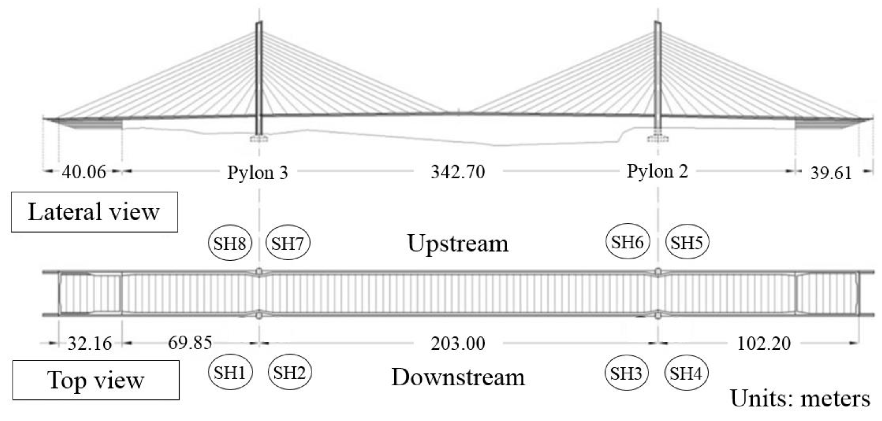
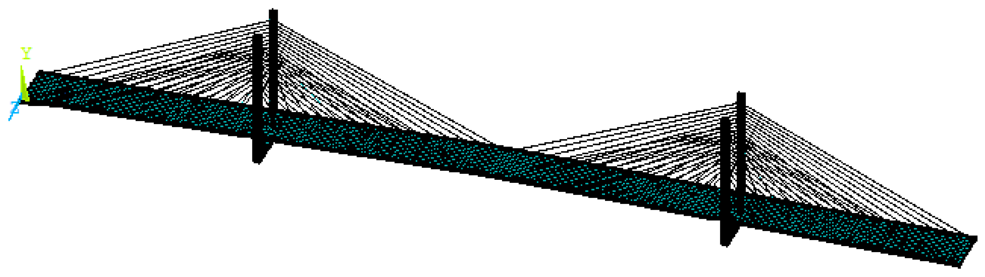
Thus, in this work, an entropy wavelet analysis is carried out, which gives rise to the new EWM, which improves the WEAM, making it more efficient for damage identification in highway bridges via the use of the vibration data obtained from numerical simulations, based on the finite element model of the Rio Papaloapan Bridge (RPB) in healthy conditions and with diverse damage scenarios (different locations and damage severities), which was calibrated by taking the vibration monitoring data of the real bridge in operation as reference. Moreover, the vibration data acquired from the real-life RPB in its healthy condition and with a removed cable are used to validate this new method in an experimental manner. Therefore, with the implementation of the algorithm based on the Shannon entropy, it is possible to optimize the WEAM in order to have a new, more efficient, and simple method (EWM) for the identification of damage in highway bridges, allowing us to obtain results for damage detection and localization with precision and with very low computing time. This has allowed us to simplify the original method, which involves more stages and analyses that require a high computational load and personnel with knowledge on the topic. It was demonstrated that the EWM is capable of eliminating 36% of the steps required to apply the WEAM, the damage location precision is increased 0.11%, and, above all, the computing time required to provide results is reduced by 5.67 times. For both methods, a Dell^© Optiplex 980^© computer with a 2.93 GHz Intel© Core^© i7^© processor, 1.81 TB of hard drive capacity, 8.00 GB of RAM, and Windows 10 Pro^© operating system were used; whereas, the corresponding codes to post-process the signals were written in MATLAB^© (R2017a). Thus, the results of the EWM application, both numerically and experimentally, were successful, and, therefore, this new method is presented as a promising alternative to be implemented permanently in the most critical bridges of a specific country in order to gain knowledge regarding their structural conditions, avoiding tragic collapses.

2. Description of the Rio Papaloapan Bridge (RPB)

The RPB is a cable-stayed bridge situated in Veracruz, Mexico, with 407.21 m of total length and 203 m of main span. This bridge began operating in 1994, and has 8 semi-harps (SH) with 14 cables for each one, making a total of 112 cables; the shortest cable is recognized with the number 1, whereas the longest cable is recognized with the number 14. In Figure 1, some pictures of the RPB are presented, while, in Figure 2, the corresponding layout of the RPB is included, showing the general dimensions and identifications of semi-harps.

2.1. Finite Element Model

The numerical model of the RPB was developed via the finite element method (FEM), using the software ANSYS^© (V 14.0) for this purpose. The elements utilized to create the model were SHELL181 for the deck; BEAM188 for pylons, main girders, and transverse girders; and LINK180 for the stay-cables. All the dimensions, material properties, and boundary conditions were carefully considered and assigned to each element of the model, resulting in a final model of 7365 elements and 8053 nodes (see Figure 3). This model was developed with the possibility of including damage in the deck by reducing the cross-sectional area of any specific part of the deck, with different severities of damage (width and depth).

In order to obtain the vibration responses of the RPB numerical model under different health conditions while a moving load (simulating a vehicle) crosses the bridge, a load was implemented on the deck of the model at an initial defined node, moving from node to node (at a specific constant speed and in a straight line) through the deck until reaching the final node, following the route that a vehicle would take along a certain lane of the bridge. Lastly, the transient responses are obtained for the different scenarios simulated, and the corresponding data series (time vs. acceleration/displacement) are exported to be post-processed with the EWM to detect/localize damage.

2.2. Experimental Tests

After a major failure occurred in an upper anchoring element which was used to attach a cable to the corresponding pylon of the RPB, a broad-scope remote monitoring system was installed in this cable-stayed bridge in 2013, which was configured with three subsystems, including sensors, local monitoring, and photovoltaic [1]. As part of the maintenance program, the RPB was monitored in 2019 under two different integrity conditions as follows: a healthy bridge, and a damaged bridge without cable No. 6 from SH3, which was removed in order to inspect its corresponding upper anchoring element.

The respective vibration data of the RPB deck in vertical direction were measured for both integrity conditions via the use of complementary instrumentation, consisting of twelve ±2 g tri-axial MEMS wireless accelerometers model G-Link^®-LXRS^®, fabricated by LORD MicroStrain^®. The sensors were installed on both sides of the bridge (downstream and upstream) on the deck of the semi-harps SH3, SH4, SH5, and SH6, as can be observed in Figure 4 via the 12 blue dots (S1–S12). The date were acquired first for the healthy condition and then for the damaged condition. The damage scenario is represented in Figure 5, where the red line indicates the cable which was removed. For both scenarios, the bridge was monitored for 1800 s, establishing a sampling frequency of 64 Hz, for a total of 115,200 samples per sensor. Moreover, the dynamic responses were divided into segments of 1 min per one, thus generating 30 tests for each case.

3. Damage Identification Methodology and Their Fundamentals

This section introduces the mathematical concepts underlying the proposed method, named EWM, for identifying damage in bridges. Specifically, it describes the two theoretical fundamentals of the algorithms on which this new method is based (the Shannon entropy and the CWT).

3.1. Shannon Entropy

Entropy is commonly associated with the amount of disorder or order; the greater the entropy, the greater the disorder or chaos [58]. The Shannon entropy index (SEI) is a nonlinear measure developed by Claude E. Shannon [57], the father of the entropy theory, and serves to quantify the complexity and uncertainty found in a time signal. In particular, the SEI has demonstrated suitability for analyzing signals in the time domain with noise and non-stationary properties, such as those measured in civil structures, especially large ones [59]. This makes it a reliable tool with which to evaluate the health status of civil structures, largely since its value can vary depending on the alterations or changes measured in the dynamic response [60].

To measure the complexity of a timing signal X, the SEI is calculated as follows:

$$SEI\left(X\right)=-{\sum }_{i=1}^{K}p\left(x_i\right){\mathrm{l}\mathrm{o}\mathrm{g}}_2\left[p\left(x_i\right)\right],$$

(1)

where p(x_i) represents the probability that a time signal X can take according to its results, x₁, x₂, x₃, …, x_K.

As an illustrative example, the SEI can be obtained via a Bernoulli trial [61], which is a randomized experiment named in honor of Jakob Bernoulli, in which only two results can be obtained, being labeled as either a success or a failure, see Figure 6. From the point of view of probability theory, these trials are modeled via a random variable x that can take only two values, 0 and 1. Typically, 1 is used to represent success. Therefore, if p is the probability of success, then the entropy depends on the probability p(x = 1) that x can take the value 1. When p(x = 1) = 0.5, all possible outcomes are equally probable, meaning the result is not very predictable, and that the entropy is maximum.

In the last decade, the Shannon entropy has been applied for different purposes, including the evaluation of the health condition of structures [44,45]. The Shannon entropy measures the uncertainty in a random variable [57]. Therefore, this can be a reliable indicator to identify damage in a civil construction, since the vibration signals change according to the damage level, consequently generating a variation in the Shannon entropy magnitude [44,45]. Therefore, since the Shannon entropy is associated with chaos, this helps to determine in which parts of a signal there is more or less chaos, associating high levels of chaos or entropy with an important phenomena or critical situations in the signals.

3.2. Continuous Wavelet Transform

One of the most utilized wavelet transforms (WT) is the continuous wavelet transform (CWT), which applies a variable-sized window method into a time-domain signal in order to convert it to a time-frequency diagram (see Figure 7).

First, a mother wavelet (MW) is selected, and this base signal is used to continuously create a wavelets’ family by means of the translation and dilation of the MW itself along the entire signal to be analyzed. Then, this process is implemented sequentially, and, in this way, it is possible to assess the similarity between the MW chosen and each segment of the complete signal to be examined throughout the entire time. As a consequence of this process, the discontinuities contained in the analyzed signal will generate high CWT coefficient magnitudes, which could be related to damage [62].

It is important to mention that there is a wide range of types of MWs, and the correct selection depends on the application in which it is required to be used, following a trial-and-error process to find the most convenient one.

Thus, if a MW is considered [63]

$$\psi \left(t\right)\in L^2\left(\mathbb{R}\right),$$

(2)

its two fundamental properties are zero mean and its normalized nature. These properties are mathematically represented as follows:

$${\int }_{-\infty }^{\infty }\psi \left(t\right)dt=0$$

(3)

$${\parallel \psi \left(t\right)\parallel }^2={\int }_{-\infty }^{\infty }\psi \left(t\right){\psi }^{\mathrm{*}}\left(t\right)dt=1.$$

(4)

Then, considering that it can be translated and dilated, the MW can create a basis set, as indicated below:

$${\left.\left\{{\psi }_{s,u}\left(t\right)=\frac{1}{\sqrt{s}}\psi \left(\frac{t-u}{s}\right)\right\}\right|}_{u\in \mathbb{R},s\in \mathbb{R}+}.$$

(5)

where $u$ is the translataion parameter and $s$ is the scale parameter. Thus, the CWT is the coefficient of the base ${\psi }_{s,u}\left(t\right)$, that is

$$Wf\left(s,u\right)=〈f\left(t\right),{\psi }_{s,u}〉$$

(6)

$$Wf\left(s,u\right)={\int }_{-\infty }^{\infty }f\left(t\right){{\psi }^{\mathrm{*}}}_{s,u}\left(t\right)dt$$

(7)

$$Wf\left(s,u\right)={\int }_{-\infty }^{\infty }f\left(t\right)\frac{1}{\sqrt{s}}{\psi }^{\mathrm{*}}\left(\frac{t-u}{s}\right)dt$$

(8)

In this way, by using this transform, a three-dimensional colored CWT diagram can be obtained with good resolution for all the parameters (time, scale, and coefficients) from a one-dimensional time signal; however, obtaining these diagrams with a high resolution and with wide ranges of scale and time will require a high computational consumption time, even more for long bridges and for vehicles crossing with low speed.

3.3. Entropy-Wavelet Based Method (EWM)

The EWM, as explained previously, was developed from the need to make the WEAM more efficient for damage identification in highway bridges, in such a way that the necessary stages and the computing time required to apply the WEAM could be significantly reduced [1], but without losing its precision in the damage identification. Figure 8 illustrates the steps of our proposed, the EWM method, and the WEAM method.

Thus, the EWM was applied to evaluate the health condition of the RPM bridge is presented in Figure 8, and this consisted of recording the vibration signals at different points along the bridge deck while a vehicle crosses it. Subsequently, the average SEI corresponding to the CWT coefficients of the current case to be analyzed is calculated considering the different measurement points and a wide scale range. Next, starting from the lowest point of the SEI, the useful scale range is defined to identify the damage, and the average curve of the CWT coefficients is obtained considering the selected scale range and the different measurement points. Finally, the curve obtained from the CWT coefficients is compared with the corresponding curve of the healthy case (baseline), and, if there is damage, a sudden increment in the amplitude of the CWT coefficients will be observed in the position of the damage for the current case. This will not happen for the healthy case, since the case without damage will exhibit a curve that will tend to be very flat and of low amplitude.

The step-by-step application of the EWM for the detection and localization of damage in bridges is as follows:

• Instrument the bridge with vibration sensors distributed proportionally along the deck.
• Obtain vibration responses for the healthy bridge (baseline) and for the current condition of the bridge while a vehicle or vehicles cross the bridge.
• Obtain the average SEI for the CWT coefficients of the current case to be analyzed, considering the data from all the measurement points and a very wide scale range, allowing SEI results outside of the effect zone of the structure natural frequencies.
• Define the most useful CWT scale range for damage identification from the lowest point of the SEI value (end of the effect of the structure natural frequencies) and upwards.
• Apply a suitable filter to remove as much noise in the signals (Savitzky–Golay filter; order: 2, window length: 19) and eliminate any edge effects by extending the signals on both sides. It should be noted that this step is not entirely necessary, since in the results presented in Section 4, it can be observed that even without filtering or extending the signals, the identification of damage is possible and very evident. However, it is recommended to filter and extend the signals, so that the detection and location of damage is even clearer. Likewise, the most appropriate MW must be used throughout the application of the EWM, which corresponds with the one previously defined via the WEAM (Mexican hat for the RPB).
• Obtain the average value of the CWT coefficients for the selected scale range and for the different measurement points.
• Compare the curve obtained in the previous point with the corresponding curve of the healthy case. If there is damage, the magnitude of the CWT coefficients will increase suddenly at the location of the damage, which will not happen for the healthy case, since the healthy case will demonstrate a curve of low amplitude without significant increments at specific positions.

Thus, comparing this new methodology, EWM, with the WEAM presented in [1], the simplification of steps achieved with the EWM is evident (from 11 to 7 stages); however, it should be noted that the steps that were eliminated with the EWM are the ones that consume the most computing time with the WEAM. Therefore, damage identification becomes faster and more efficient with the EWM and without sacrificing the precision in damage detection/localization, as will be demonstrated in the next section of this article.

4. Numerical Results and Analysis

In this section, the EWM is numerically validated through simulations with the finite element model previously described. For this purpose, the EWM is applied in the FEM model of the RPB in its healthy condition, as well as with different damage scenarios. The results indicate that the detection and localization of all the damage cases is possible with the EWM in a quick, accurate, and efficient manner.

Since, in this article, the EWM is presented for the first time, in this section, several diagrams will be shown and analyzed in detail, which will allow for the sequential observations of how the idea of making the WEAM more efficient arose, by implementing an algorithm based on the Shannon entropy in order to give way to the EWM. Moreover, the EWM was applied to identify diverse damage conditions, and the corresponding results/diagrams will be also presented.

The most important challenges that led to the development of the EWM were the reduction of the steps required to apply the WEAM and the reduction of the computing time necessary to obtain the results, which allow for the detection and localization of damage without losing any precision. Therefore, since these are processes that involve a significant computational burden which are related to other stages, it was identified that the definition of the CWT scale range, useful for identifying damage with the WEAM via the use of colored 3D CWT diagrams, is the most critical stage of that method (stage 5 in [1]), along with the generation of new colored 3D CWT diagrams to identify damage in the area of interest (stage 8 in [1]).

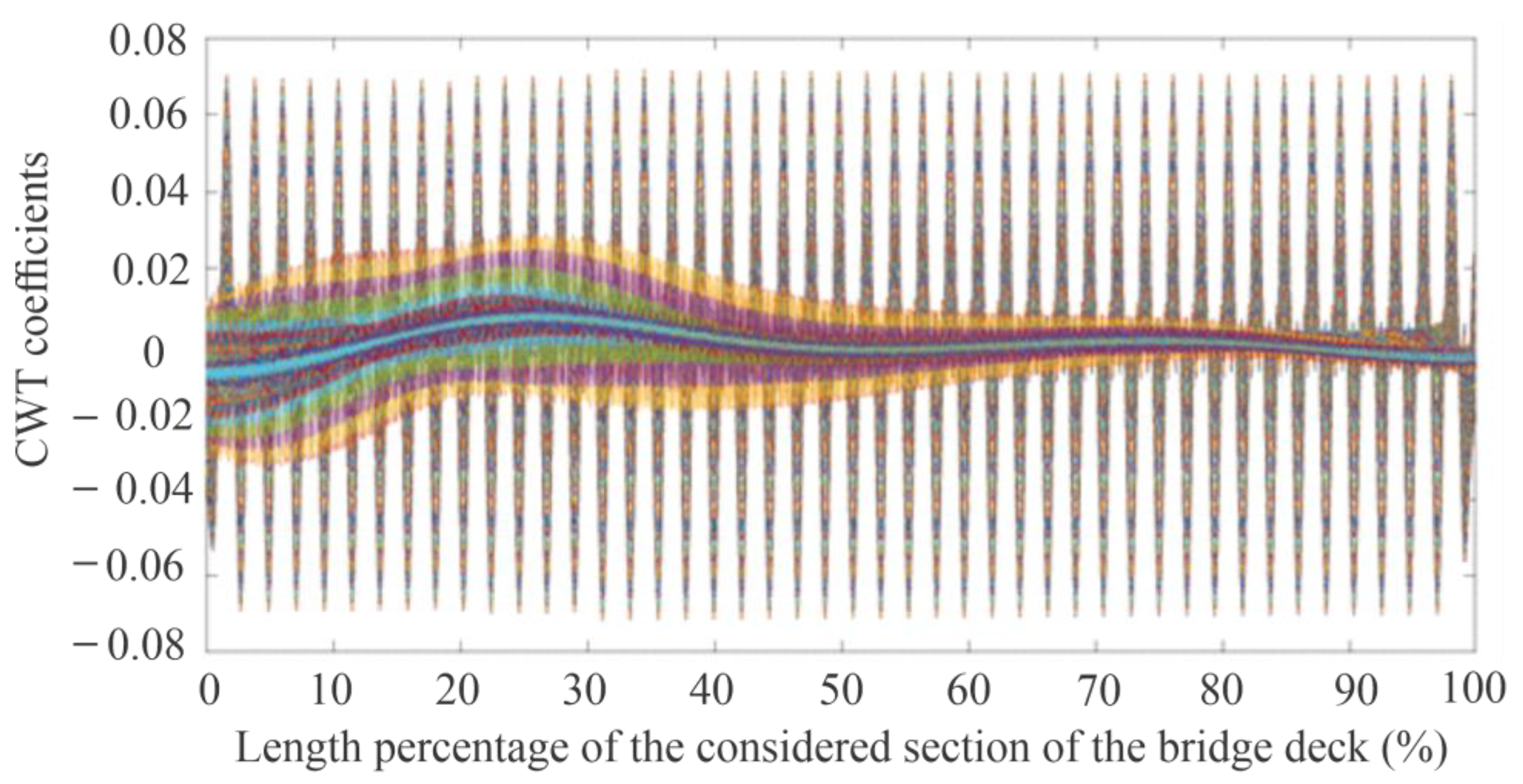
Thus, considering the stages of the WEAM, which were described in detail in [1], seven of those steps were eliminated via the EWM (steps 4, 5, 7, 8, 9, 10, and 11); that is, 64% of the WEAM stages were eliminated and replaced with a few steps requiring low computing time consumption. It should be noted that around 95% of the computing time needed to obtain the results via the application of the WEAM and determine the health condition of the analyzed structure relates to the stages 5, 7, 8, 9, and 10, and all of them were eliminated with the EWM. Consequently, the EWM began to be designed, processing the corresponding data from the numerical simulations with the scenario of the damaged bridge, with an intermediate severity damage on the deck at 25% of the length (simulated by reducing 30% the area of the cross-section at 25% of the 203 m length of the bridge deck between towers), and the CWT coefficients were obtained for each scale value, from 1 to 1000, measuring at 25% of L. In the corresponding diagram that was obtained (see Figure 9), it can be observed that it is difficult to detect damage due to the large number of curves. However, it can be noted that there are certain curves with magnitude increments of CTW coefficients around 25% of L. Therefore, it is necessary to define what scales these curves correspond to, discarding those that are not useful.

To clarify the diagram shown in Figure 9, the CWT coefficients were obtained again for the scale range from 1 to 1000, but now with increments of 50, and the corresponding results are presented in Figure 10. Thus, in Figure 10, it is possible to observe that most of the curves that are not useful for detecting damage no longer appear, while a significant number of the useful curves that suggest the existence of damage at 25% of L are preserved. Therefore, for this analyzed scenario, there are more useful curves than there are curves that do not reveal the presence of damage.

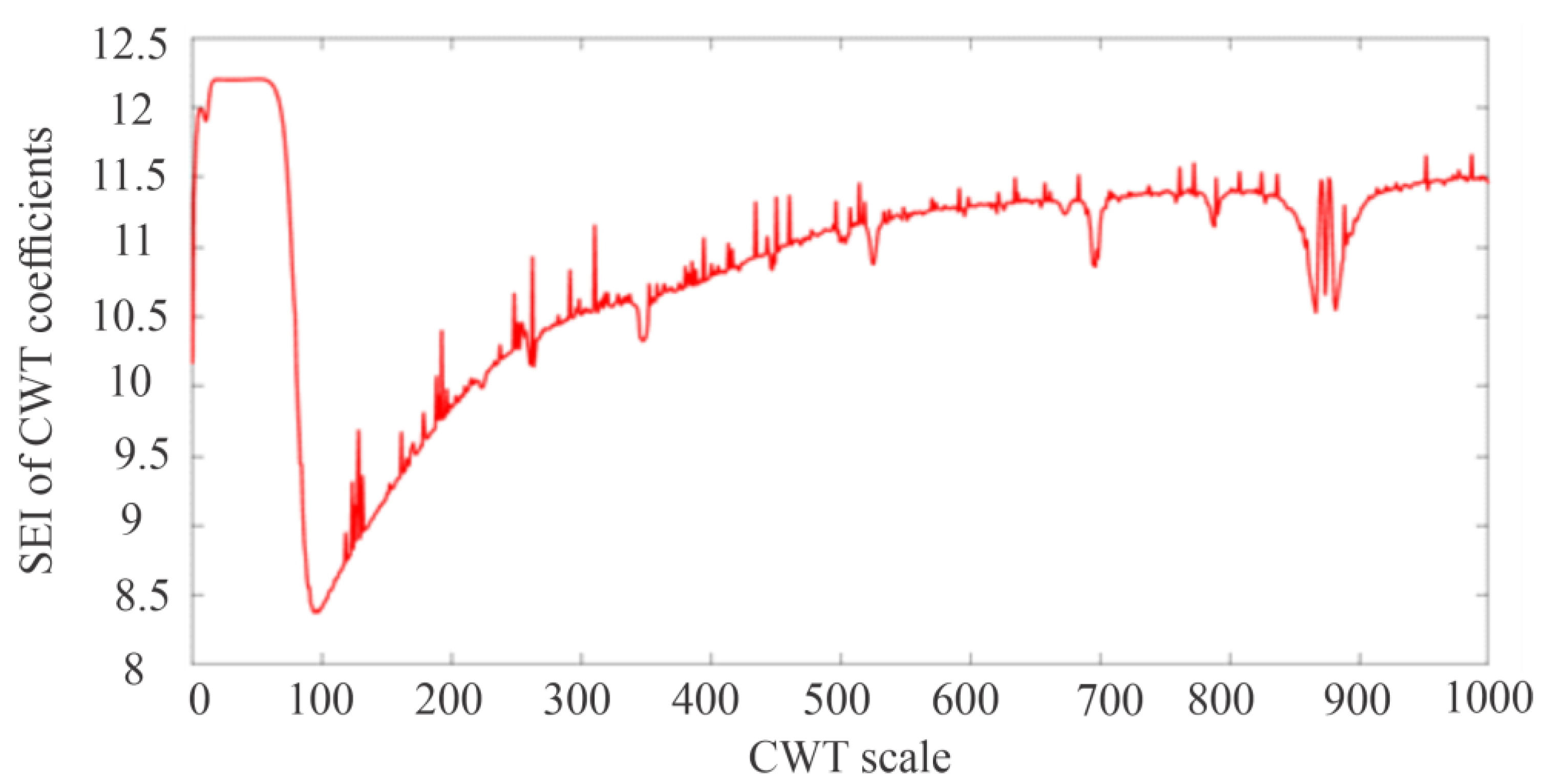
Therefore, in order to have a reliable parameter that allows for the systematic defining of the useful scale range to identify damage without the need of obtaining CTW coefficient curves for different ranges and increments of scale, an algorithm based on the Shannon entropy was implemented (see Section 3.1, Equation (1)). In this way, the average SEI for the CWT coefficients (entropy–CWT diagram) considering all of the measurement points (25%, 50%, and 75% of L) of the current scenario and the same wide scale range (1 to 1000) and scale increment used for the diagram in Figure 9 is obtained. 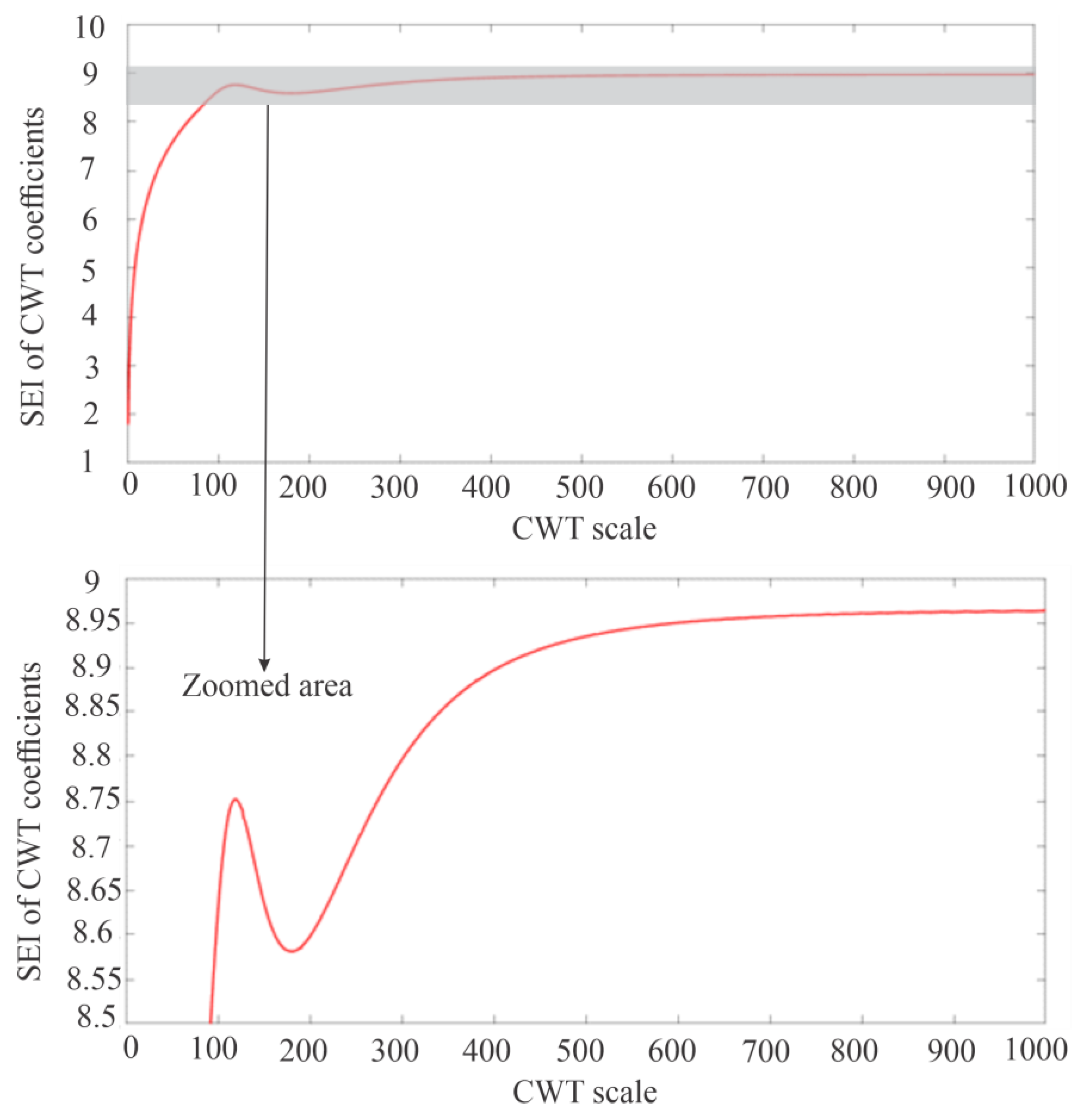Thus, in Figure 11, the respective results of the average SEI can be observed, where three zones are clearly noticed.

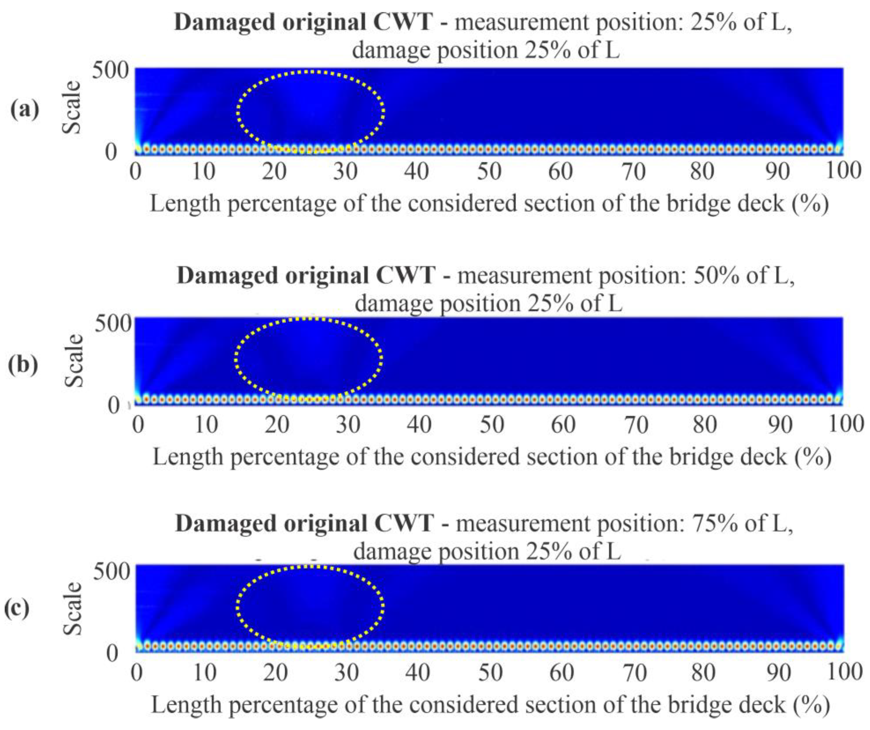
SEI zone 1: This has a scale range from 1 to 52, and the maximum SEI value can be located. In this zone, the effects of the natural frequencies of the system are present (if the WEAM were used, they would correspond to the reddish spots, indicating high CWT coefficients, as presented in the lower part of the colored 3D CWT diagrams, see Figure 12). Therefore, the high levels of chaos or entropy in this zone are due to the effect of natural frequencies, and not the effects of damage. Therefore, this zone is not useful and should not be considered to define the scale range in the EWM.

SEI zone 2: This has a scale range from 53 to 98, where the average SEI value falls from its maximum value to its minimum value. This zone indicates that the effects of natural frequencies begin to decrease until they are completely eliminated, and, on the other hand, the effects of damage have not yet appeared yet. Consequently, the chaos decreases sharply, and the minimum entropy value is due to the edge effects of the signals. This area should also not be considered to establish the scale range to detect damage.

SEI zone 3: This has a scale range from 99 to 1000, where the average SEI value gradually increases from its minimum value to a very high value close to its maximum. This zone indicates that the effect of the natural frequencies no longer exists, and the entropy increment is mainly due to the manifestation of the effects of the damage presence. Therefore, the chaos generated in this area is useful to define the scale range to identify damage.

It is important to mention that the presence of any kind of defect in any type of bridge will be clearly detectable just via the use of the SEI zone 3, since it is only in this zone that the effect of the natural frequencies, which is the most hostile and makes damage detection impossible, does not exist anymore, and the damage manifestation will be clearer. However, the CWT scale values of this zone, as well as the other two zones, will change according to the analyzed structure, and must then be determined, since the natural frequencies are an intrinsic parameter of any structure, with specific values according to its properties/geometry.

Thus, the entropy–CWT diagram presented in Figure 11 was obtained in less than 21 s (less than 7 s for each measurement point), and this is the diagram that allows for the elimination of the most critical stage of the WEAM (stage 5: generation colored 3D CWT diagrams to establish the useful scale range, which implies about 3 min and 8 s of computing time, as in Figure 12 [1], but with a scale range from 1 to 1000) and the subsequent stages that are related to this critical stage, and which consume around 95% of the WEAM post-processing time, as mentioned above. In Figure 12, the yellow dotted ellipses indicate where energy differences can be observed according to the measurement point and the damage point.

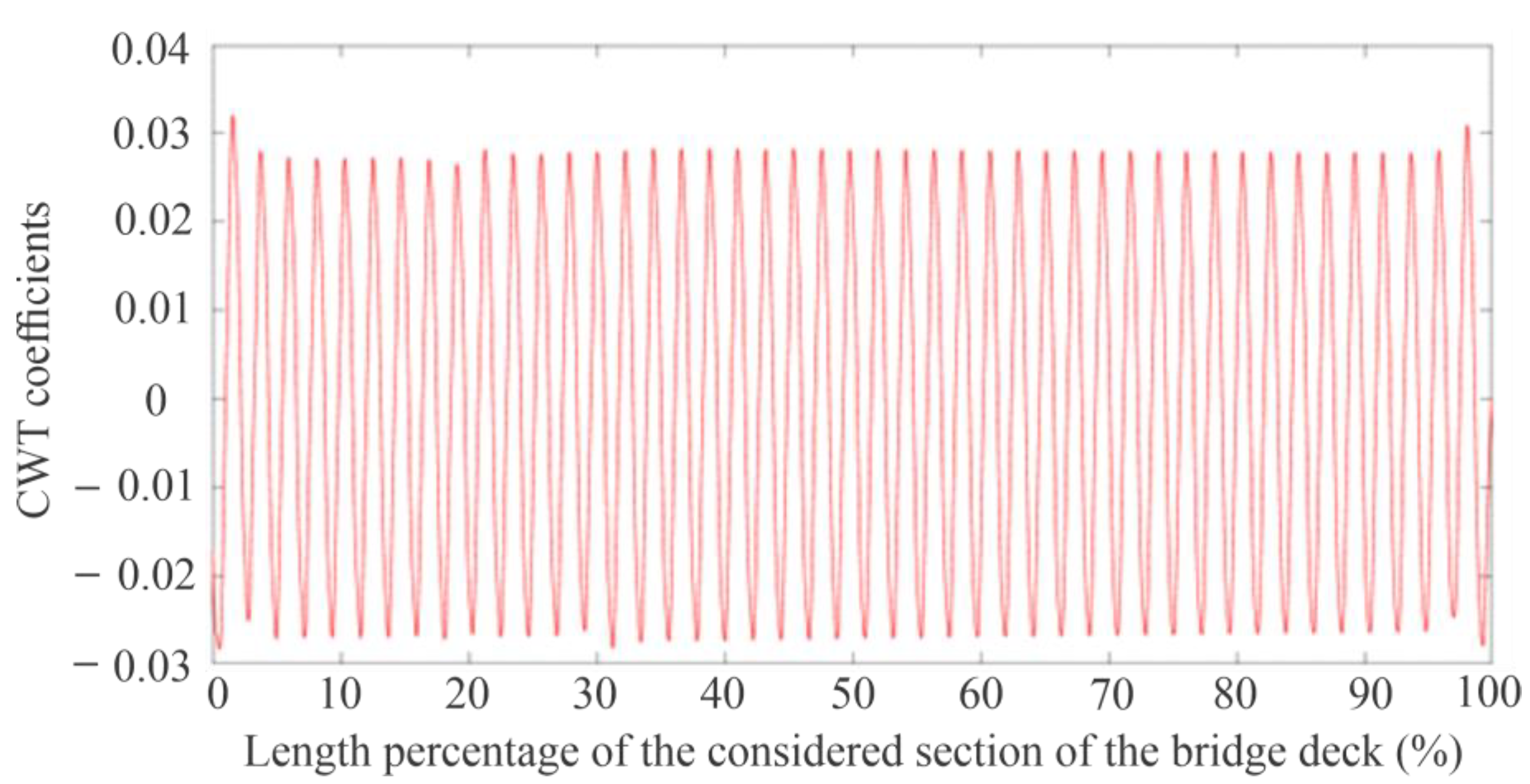
Continuing with the development of the bases that gave rise to the EWM, and taking into account the entropy–CWT diagram presented in Figure 11, the usefulness of the SEI zone 3 to detect damage is verified. To do this, the average of the CWT coefficients is obtained considering the measurement position of 25% of L and the scale range from 1 to 100 (Figure 13). This scale range includes the complete SEI zone 1 and SEI zone 2, as well as the beginning of the SEI zone 3, where the SEI is just beginning to increase due to the damage. In this way, looking at Figure 13, as expected, there is no indication of damage.

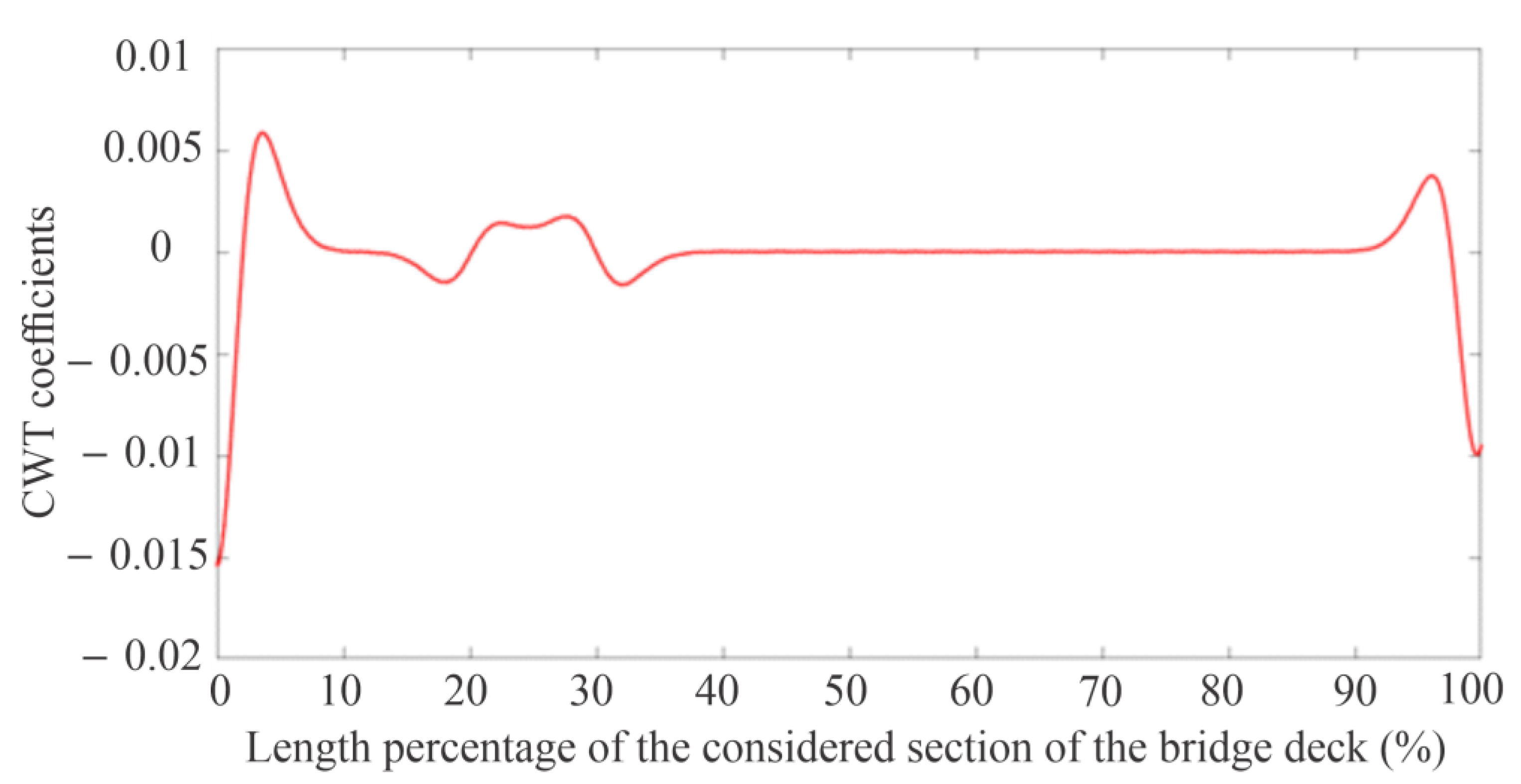
On the other hand, if the scale ranges from 101 to 181 is considered, that is, a scale range that is already completely in SEI zone 3 but still at the beginning of this zone, and the average of the CWT coefficients is obtained considering the measurement position of 25% of L, then, in Figure 14, it can be seen that the identification of the damage is already possible due to the magnitude increment of CWT coefficients around 25% of L. However, since the damage manifestation is just beginning in this zone, the edge effects of the signals still predominate, which is why the largest magnitude CWT coefficients are found at the extremes of the diagram.

Now, if the scale ranges from 181 to 500 is considered, that is, from the last scale value of the previous figure (Figure 14) and up to half of the maximum scale value considered, then the entropy increment in this range is already very significant (see Figure 11), and, therefore, the effects of the damage presence are of great significance, which can be verified by generating the corresponding diagram of the average CWT coefficients (see Figure 15).

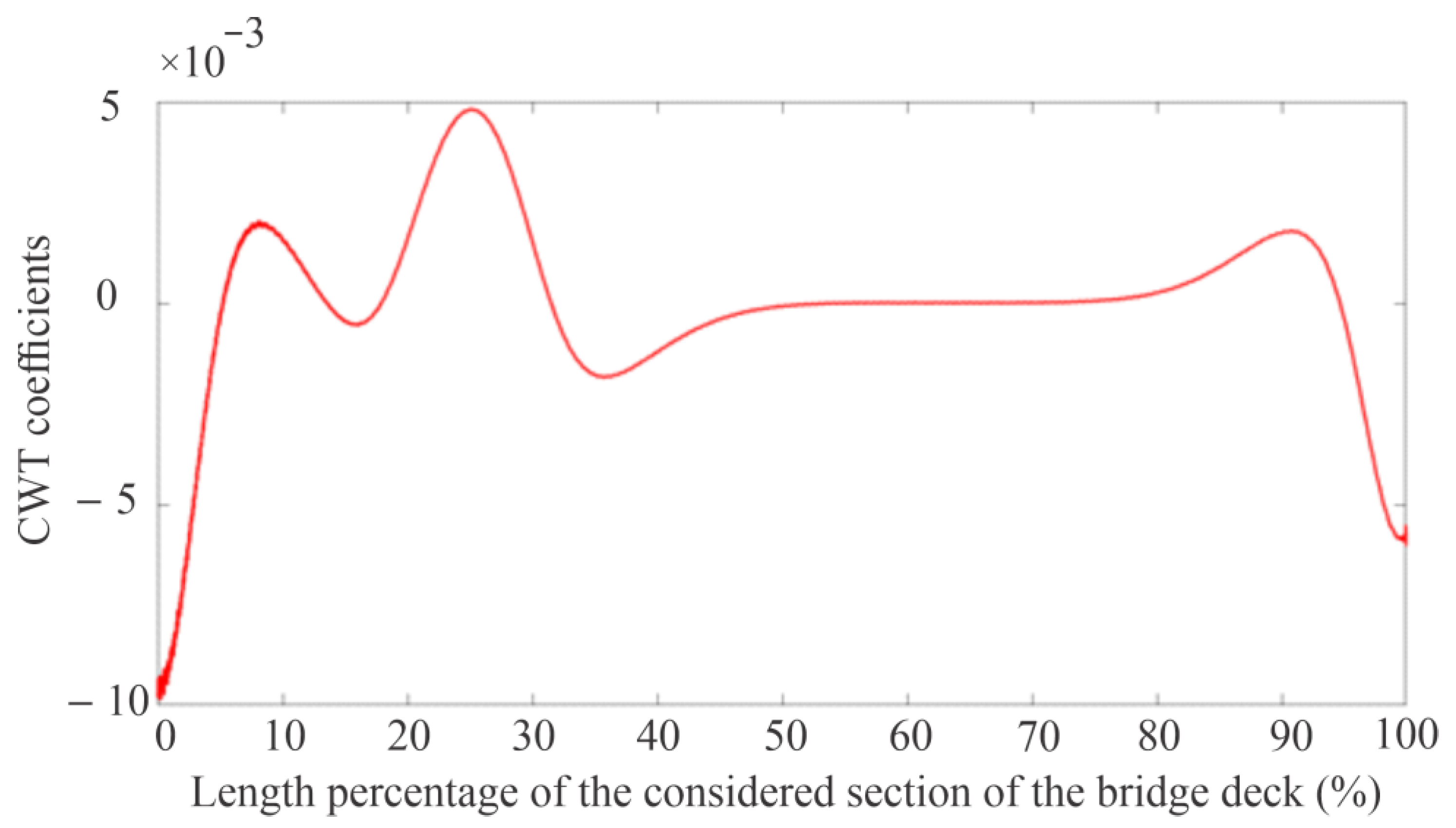
In Figure 15, it can be noted that, for this scale range of 181 to 500, the sudden increase in the magnitude of the average CWT coefficients around the damage zone is very evident, reaching its maximum value practically at the exact damage position (at 25.13% of L). Additionally, it is important to highlight that the damage effect in this region of SEI zone 3 is already very important, meaning that even the maximum value of the average CWT coefficients at the damage zone exceeds the maximum values of the CWT coefficients generated at the ends of the diagram due to the signal edge effects.

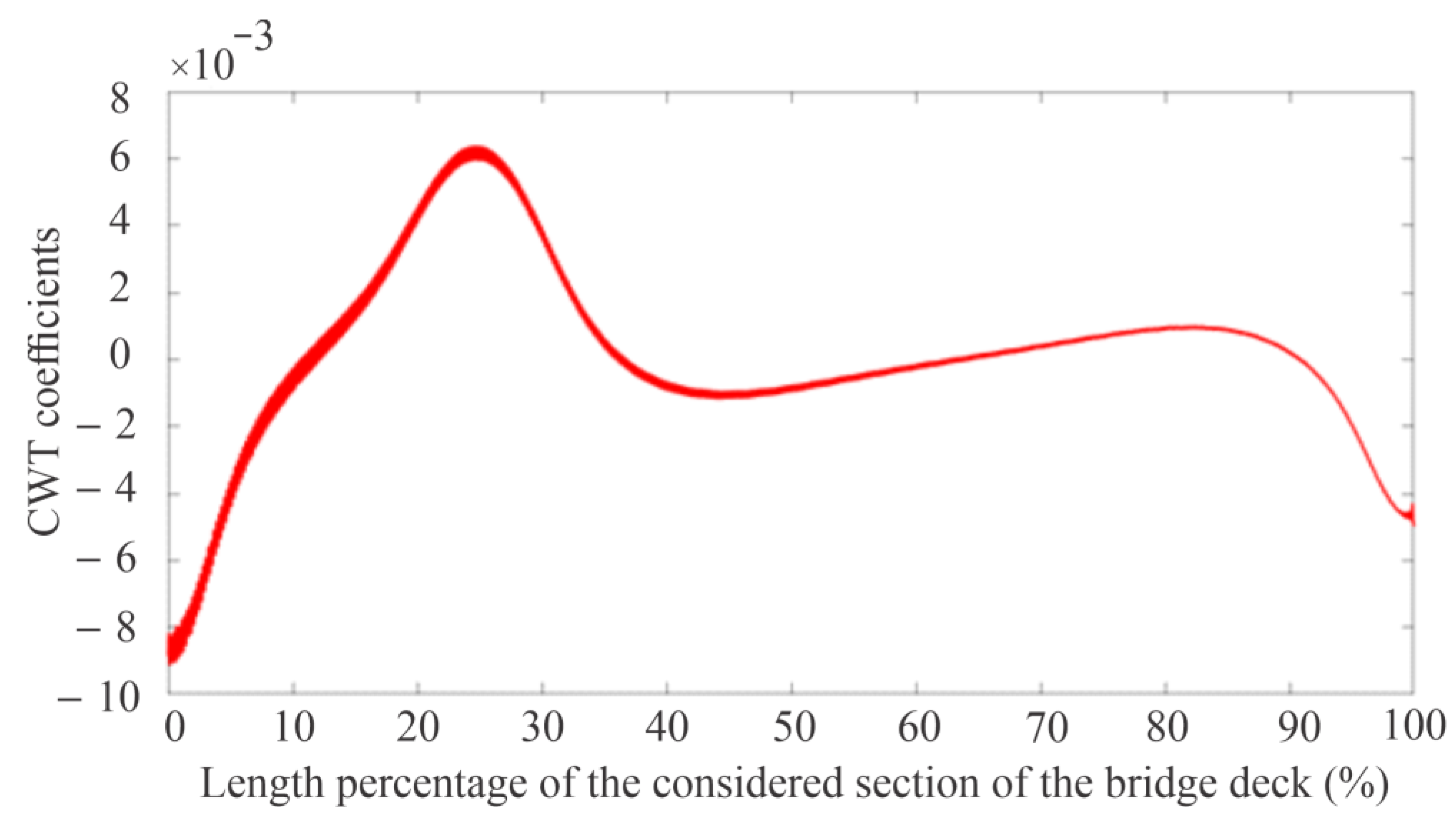
On the other hand, since it was found that the scale range, from 181 to 500, which is located in SEI zone 3, is very useful for identifying damage, this scale range is extended up to the maximum value considered in Figure 11, taking advantage of the influence of more damage effects. Then, the scale range, from 181 to 1000, is now considered, and the respective average CWT coefficients are obtained (see Figure 16). In Figure 16, it can be observed that the curve of the average CWT coefficients increased its magnitude even more in the damage region because a larger damage influence zone is considered and, therefore, the chaos or entropy of the CWT coefficients is also higher. Likewise, the precision in locating the damage is the same as in Figure 15 (99.48% precision).

The other situation that must be highlighted in Figure 16 is the reduction of edge effects, even though the signal has not yet been treated/conditioned for this purpose. This is because, by expanding the scale range, the damage effect is “strengthened”, and the edge effects of the signal are “dimmed”, so, as expected, the edge effect that is most inhibited is the closest one to the damage position; that is, the one on the left side of the diagram.

Both the diagrams in Figure 15 and Figure 16 are generated very quickly (4 s required for the one in Figure 15 and 10 s for the one in Figure 16). Therefore, the time difference between them is very small, but, with the diagram presented in Figure 16 with a wider scale range, more noticeable evidence of damage and the inhibition of signal edge effects is gained without the need of conditioning the signal (signal extension at both ends). Nevertheless, the diagram shown in Figure 15 is also very useful for identifying damage.

Thus, it is recommended to define the scale range using SEI zone 3 of the entropy-CWT diagram, locating the lowest entropy value first, and then establishing the minimum value of the scale range after the lowest entropy value in order to allow the damage to begin to manifest. The maximum value of the scale range should be defined when the SEI value of the entropy–CWT diagram practically no longer increases and remains constant. For the case currently analyzed, the scale range, from 181 to 1000, is excellent, as demonstrated in Figure 11, Figure 15 and Figure 16.

On the other hand, in order to demonstrate the reliability, efficiency, quickness, and precision of the EWM, the average CWT coefficients for the current case of damage at 25% of L is obtained for the scale range from 181 to 1000, but now considering the corresponding average of the CWT coefficients for the three measurement points (25%, 50%, and 75% of L) instead of just one measurement point at 25% of L. In this way, it is possible to verify that the EWM, like the WEAM, does not require a measurement point at the damage position, and the average of a few measurement points proportionally distributed is sufficient to identify damage.

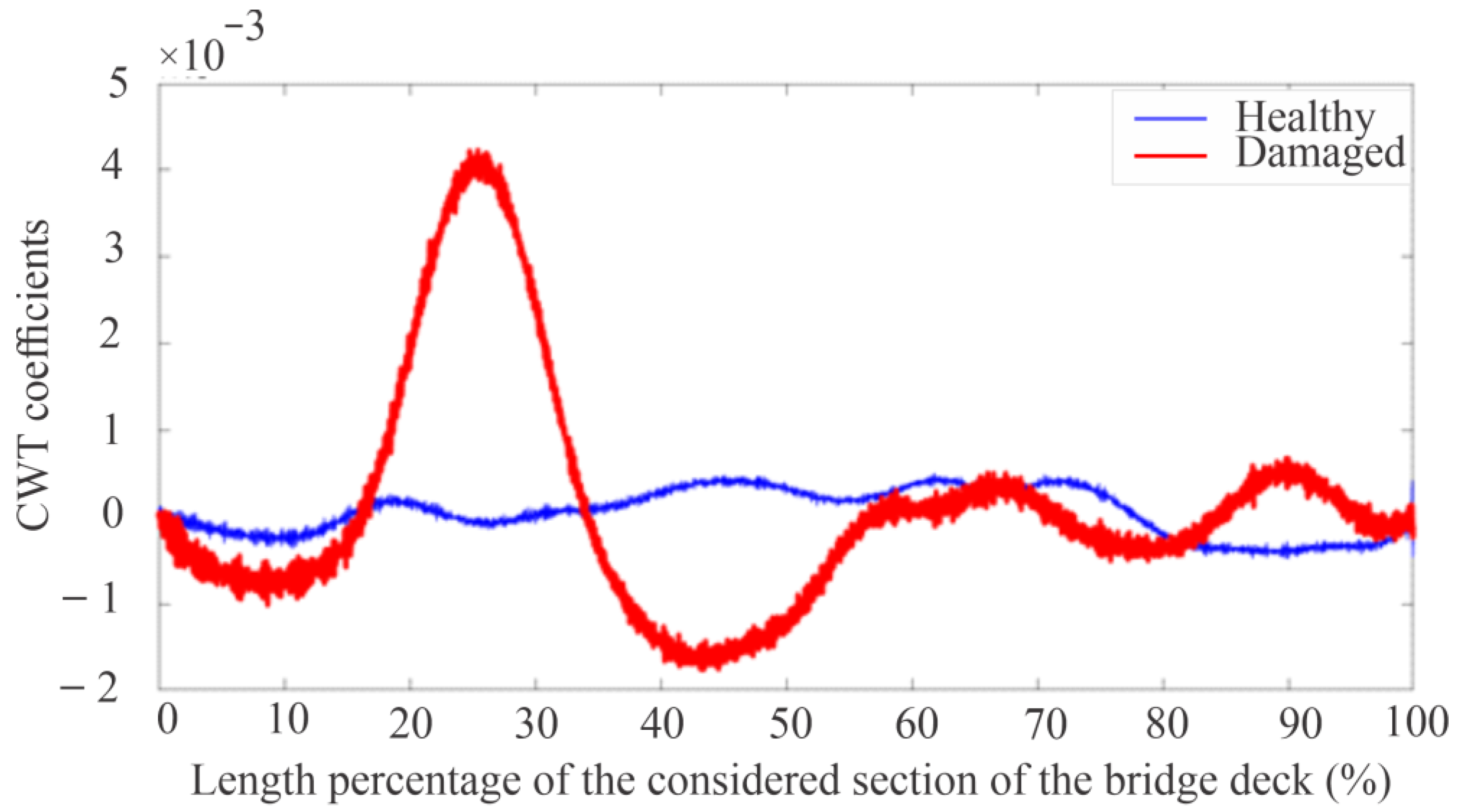
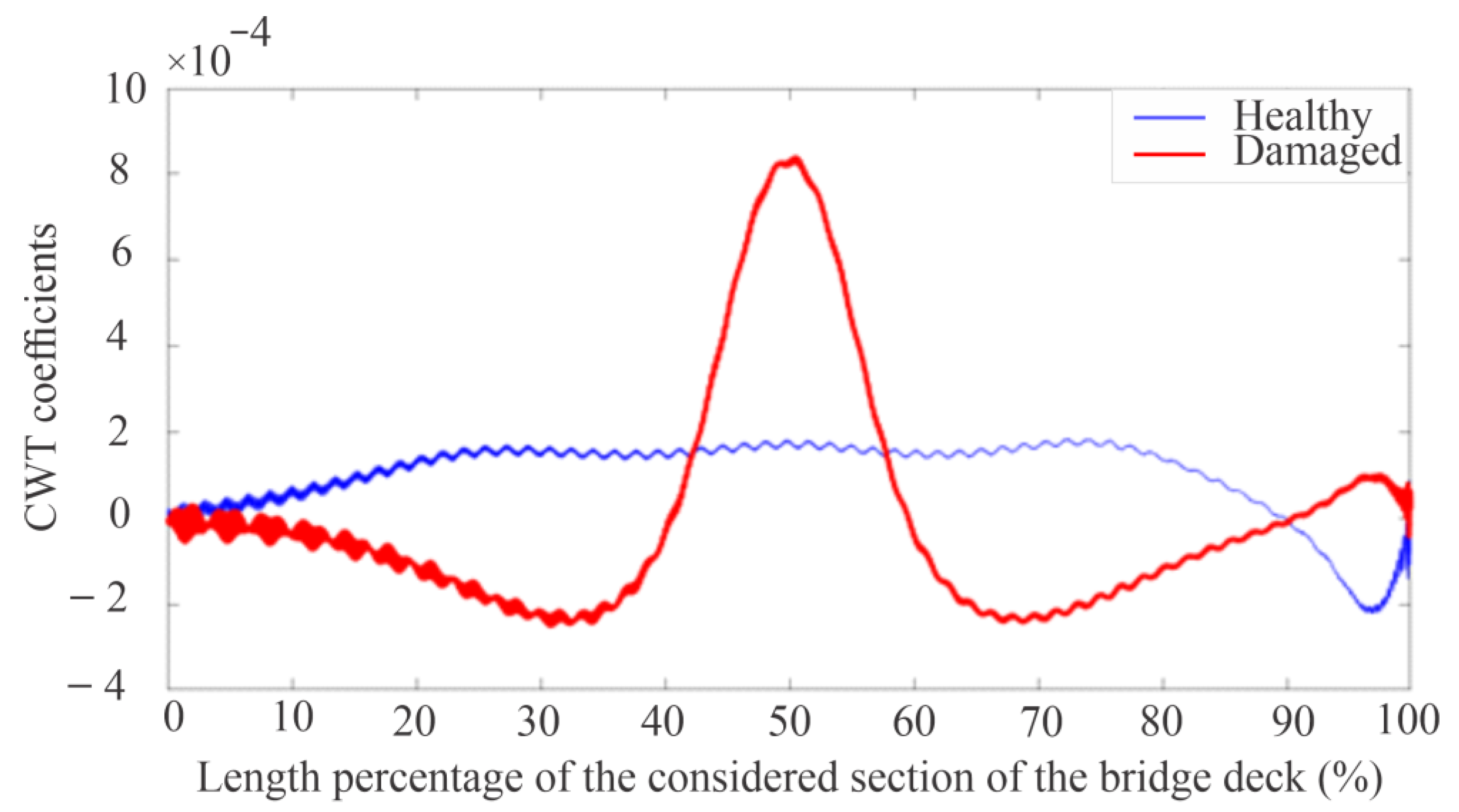
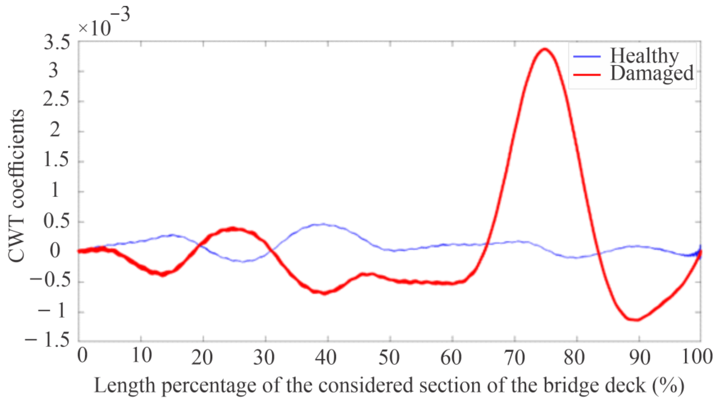
Figure 17 shows the diagram with the corresponding curve to the case mentioned in the previous paragraph, and, additionally, the respective curve of the healthy case considering the three measurement points is also included. In this figure, it can be clearly observed that the curve of the healthy case looks very flat, without any magnitude increments of CWT coefficients in specific positions; however, the curve of the damaged case, similar to the one presented in Figure 16, exhibits an evident sudden increase in the damage area, locating this defect with 99.44% precision.

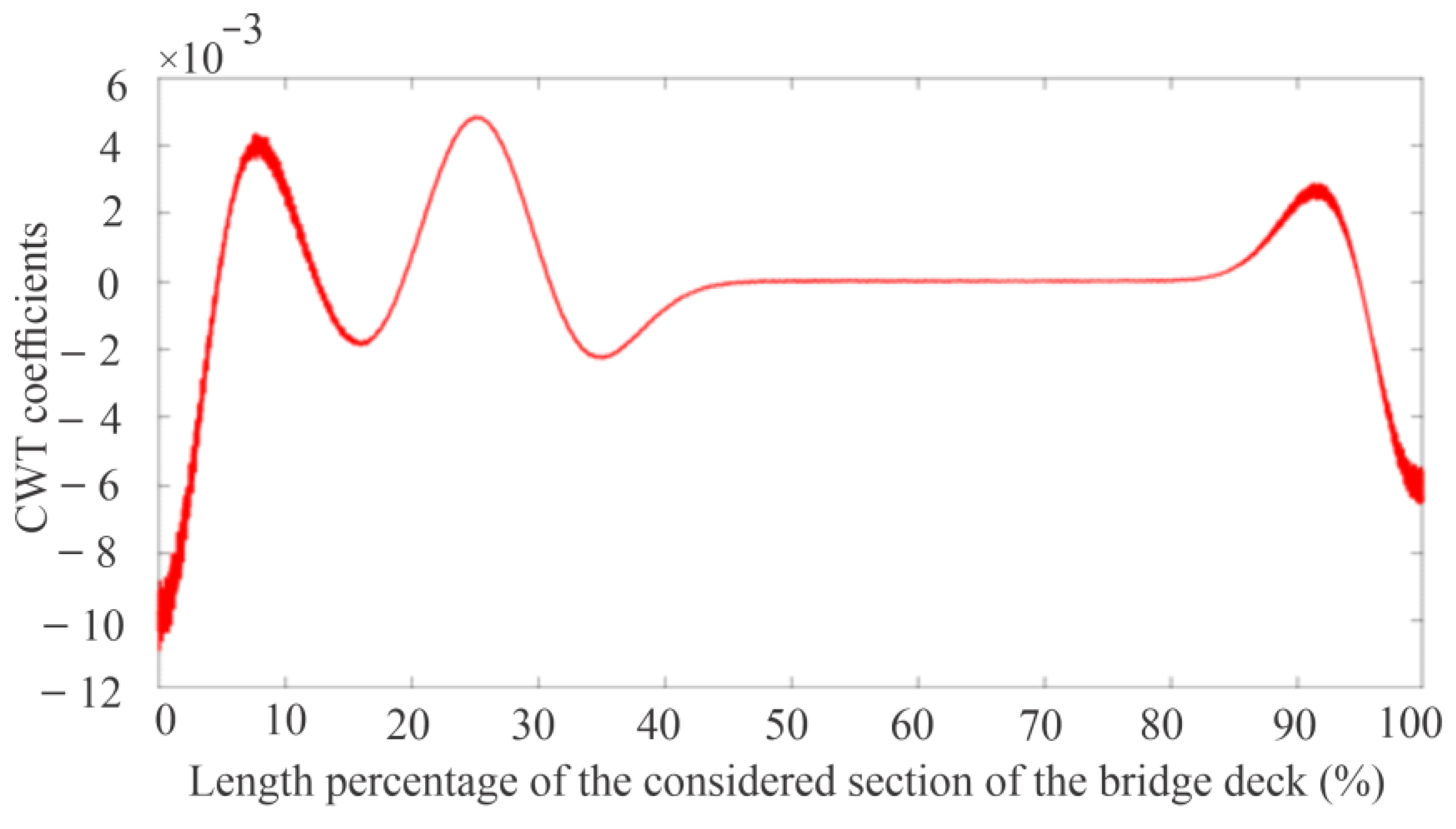
Finally, in order to have a diagram that makes the presence of the damage even more noticeable, the same diagram presented in the previous figure (Figure 17) is obtained, now eliminating the edge effects, for which, before obtaining the average CWT coefficients for the chosen scale range and considering the three measurement points, the original signals (time vs. acceleration) provided by the numerical simulations with the FEM model are extended at both ends. That is, the first and last cycles of the signals are repeated on the left and on the right sides, respectively; smoothing, in this way, the beginnings and ends of the signals in order to avoid the generation of discontinuities, which produce high CWT coefficients. The process of eliminating edge effects via signal extensions is the same as the one used for the WEAM, which is very simple, quick, and can be consulted in [1].

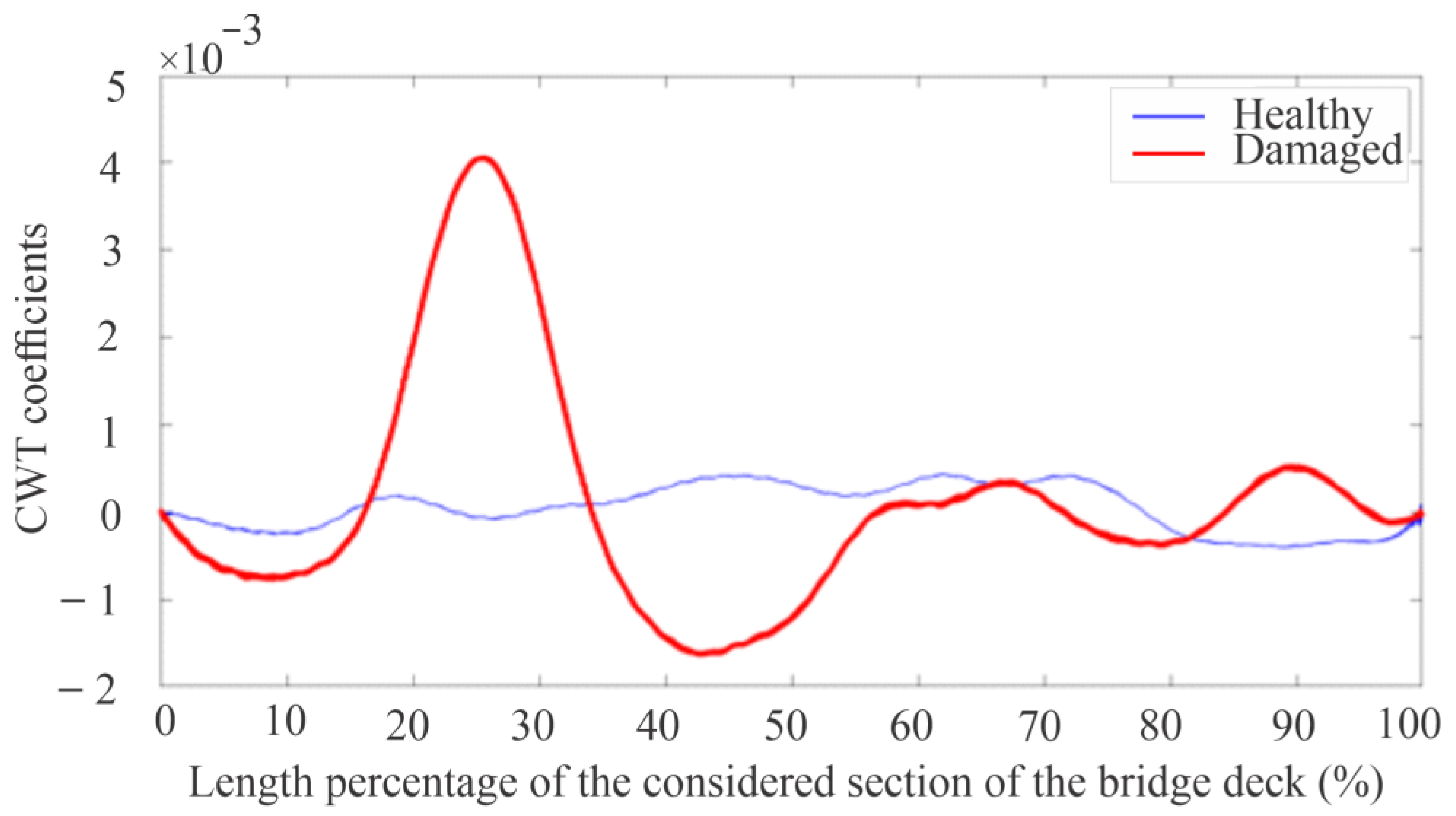
Therefore, the corresponding diagram without edge effects is shown in Figure 18. Comparing this latest diagram without edge effects with the corresponding diagram with edge effects (Figure 17), the benefit of eliminating edge effects is very evident, since the curve of the healthy case becomes even flatter because it does not contain effects that increase the CWT coefficients; there are only residual edge effects, which are almost negligible. On the other hand, for the damaged case curve, the high values of CWT coefficients in the regions where there is no damage are eliminated, and the sudden increase in the CWT coefficients is further concentrated in the damage area. In fact, the maximum value of CWT coefficients is further adjusted with the exact damage position, since the damage was located with 99.44% accuracy with edge effects, while, without edge effects, the localization precision was 99.68%.

Taking into account that these results are obtained numerically, in order to apply the EWM using signals more similar to those acquired from real-life bridges, 15% of Gaussian noise was added to the numerical signals obtained from the FEM simulations. In order to closely simulate reality, the percentage of added noise is a very high value according to what is usually considered in the literature [64].

Figure 19 shows the equivalent diagram to the one presented in Figure 18, now adding Gaussian noise to the signals before being processed. As it can be observed, despite the noise effect, damage detection is still clearly possible, and is located with 98.12% accuracy, which is an excellent percentage, especially considering the large amount of noise that was added to the signals and the extensive length of the bridge considered.

Finally, as it would occur in the practice of signal processing acquired in real-life bridges, the noisy signals are filtered to try to eliminate as much noise as possible and ensure that they are as similar as possible to the signals obtained directly from the FEM simulations before adding noise. To do this, a Savitzky–Golay filter of order 2 and window length 19 is used, in the same way that it was used for the case presented in [1] when applying the WEAM. The corresponding CWT coefficients diagram from filtered signals is shown in Figure 20, and it is possible to see that the curves are smoothed and the damage identification becomes clearer and more precise with respect to the noisy case, locating the damage with an accuracy of 98.76%, thus improving the accuracy in damage identification with signal filtering, and maintaining similarity to the original case before adding Gaussian noise (Figure 18 localizing the damage with 99.68% accuracy).

Additionally, to demonstrate the usefulness of the entropy–CWT diagram, particularly in SEI zone 3, instead of graphing the average of the CWT coefficients for the selected useful scale range (181 to 1000), the CWT coefficients for the damaged case analyzed are obtained for a single scale value that is within SEI zone 3, where the chaos increment caused by the damage is already evident. Thus, the scale value of 300 is chosen, and the CWT coefficients are plotted for this damaged case (measuring only at 25% of L) both with and without edge effects; see Figure 21 and Figure 22, respectively.

As it can be seen in both diagrams, the increase in the CWT coefficients in the damage zone is noticeable, even more so for the case without edge effects. Therefore, Figure 22 shows that the damage can be identified clearly and very accurately (99.92% accuracy in locating the damage), even with the CWT coefficients corresponding to a single scale value; however, this scale must be very well chosen based on the entropy–CWT diagram.

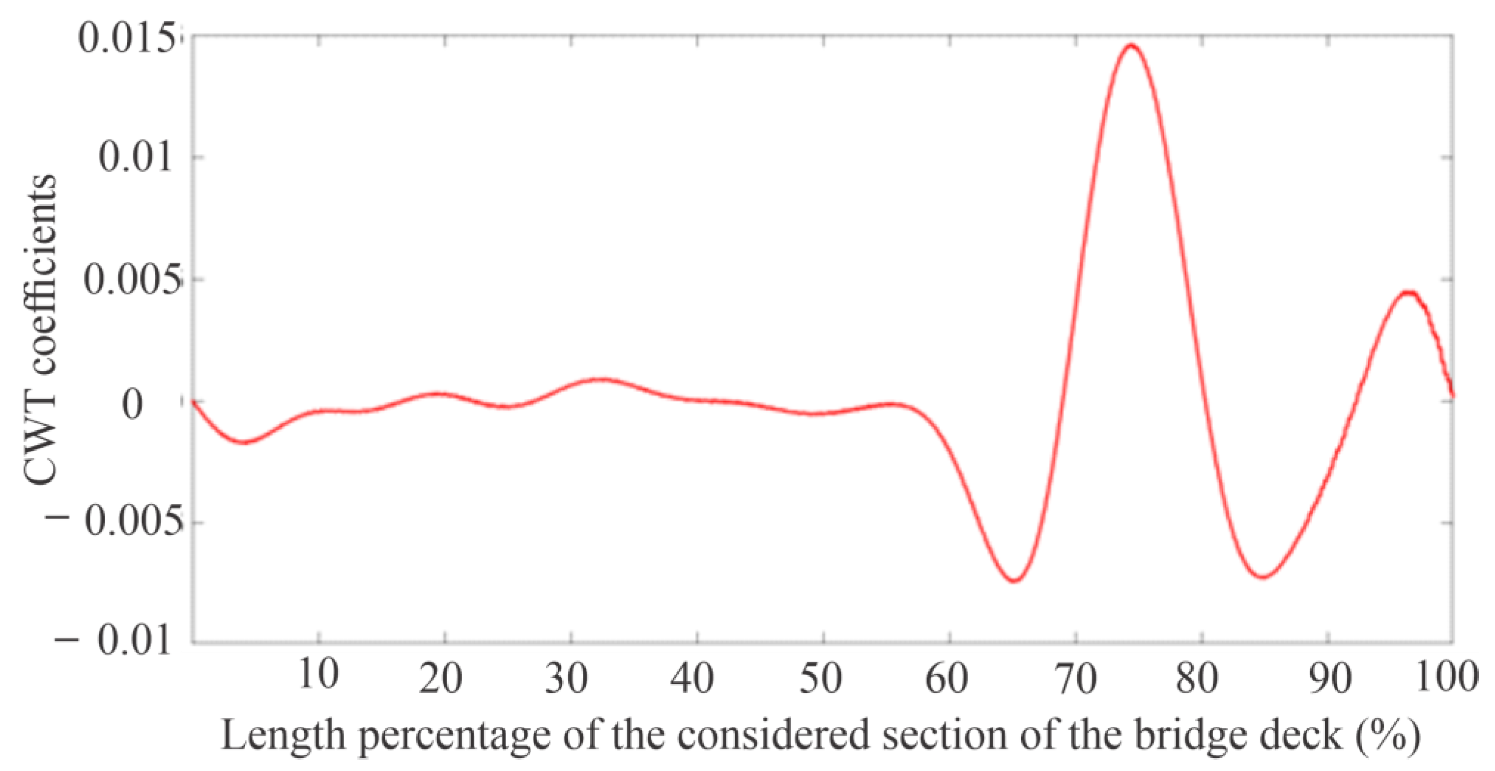
On the other hand, the EWM is applied again, as shown in Section 3.3 of this article, to demonstrate the capacity of the EWM in order to identify damage of different severities and in different positions, taking as reference the diagram shown in Figure 20, which is the final diagram obtained by applying the EWM to identify damage for the case of a bridge with intermediate level damage (30% reduction in cross-sectional area) at 25% of L. This was completed to obtain the two corresponding diagrams for the case of low severity damage (10% reduction in cross-sectional area) at 50% of L (Figure 23) and high severity damage (50% reduction in cross-sectional area) at 75% of L (Figure 24).

As it can be seen in both Figure 23 and Figure 24, the EWM is capable of clearly identifying damage of different severities in different positions with efficiency, low computing time consumption, and high precision. To obtain each of those diagrams, as well as the diagram in Figure 20, about 51 s were required, while, in terms of the precision of damage location, the damage established at 50% of L was located with 99.04% accuracy (Figure 23), the damage established at 75% of L was identified with 99.97% accuracy (Figure 24), and, previously, the damage defined at 25% of L was located with 98.76% precision (Figure 20).

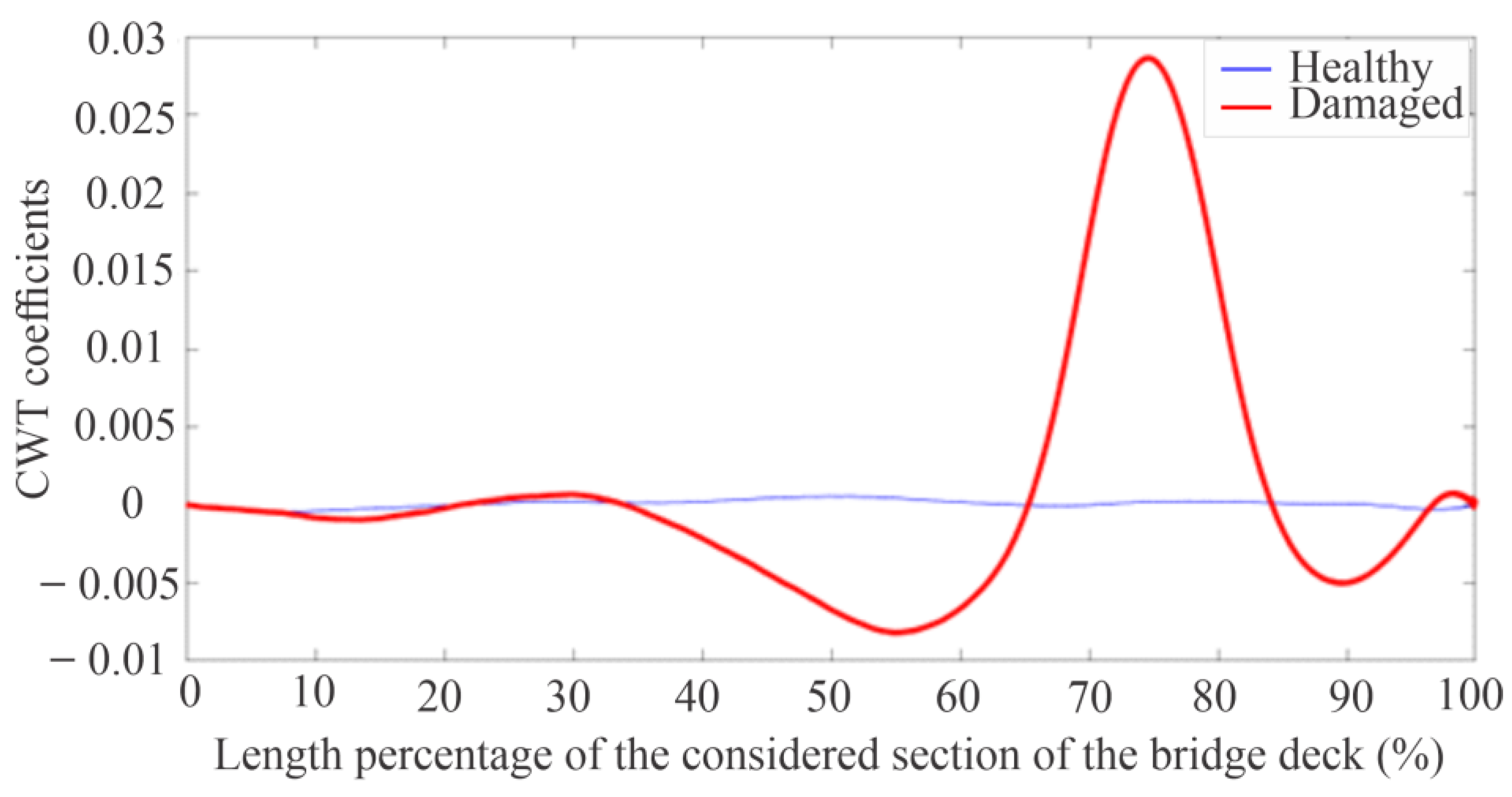
In the same way as was completed for the case shown in Figure 22, the respective CWT coefficients diagram is obtained for a single scale value (300), but now for a case with damage at 75% of L and measuring only at 25% of L. The results are shown in Figure 25, and it is possible to see that the damage was identified with high precision (99.40% accuracy) with a single scale value and with a single measurement point, which is the furthest from the damage position.

Finally, for a comparison of identical cases applying the WEAM and the EWM, the scenario presented in the last diagram of Figure 12 obtained from [1] applying the MAEW to the bridge with intermediate intensity damage (30%) at 75% of L using filtered signals is used to apply the EWM, and the corresponding diagram is presented in Figure 26. Comparing both diagrams, it is concluded that the damage located at 75% of L was identified with the WEAM with 99.68% precision (Figure 12), requiring a processing time for the signals provided by the FEM simulations of 4 min and 49 s; while, on the other hand, the EWM identified the damage with 99.79% accuracy, requiring a computation time of 51 s. In this way, the important benefits of the EWM are verified and justified, since, for the same case of the damage analyzed, the EWM identified the damage with 0.11% greater precision, obtaining results 5.67 times faster.

5. Experimental Results and Analysis

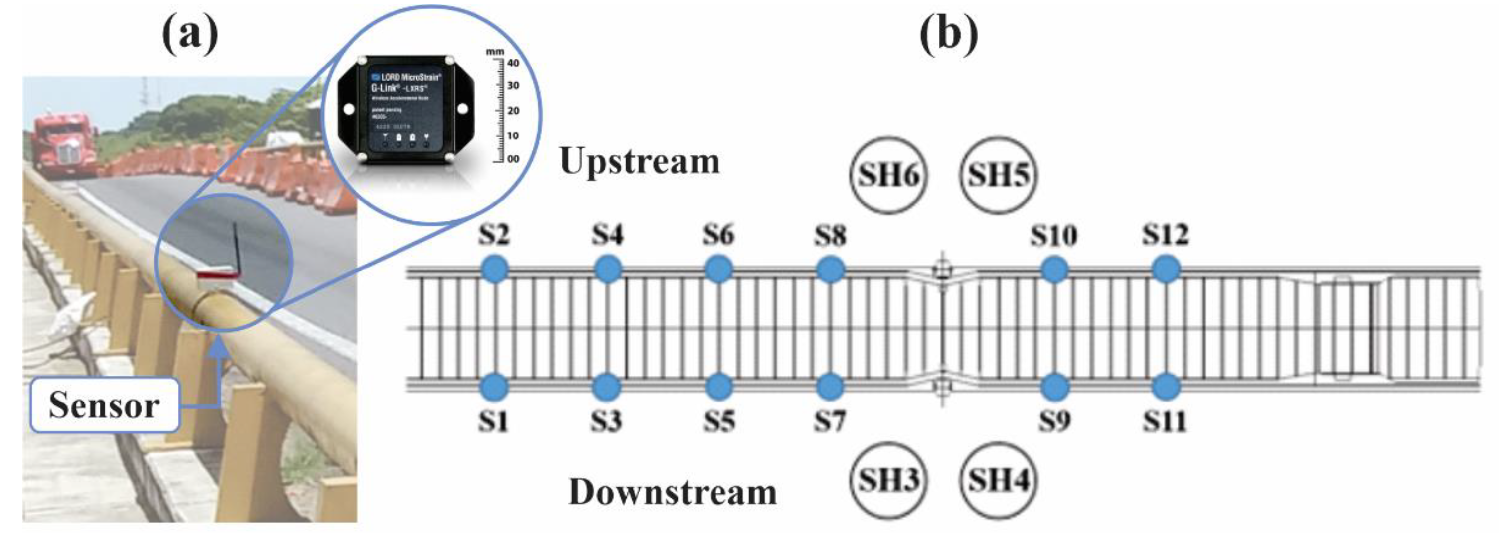
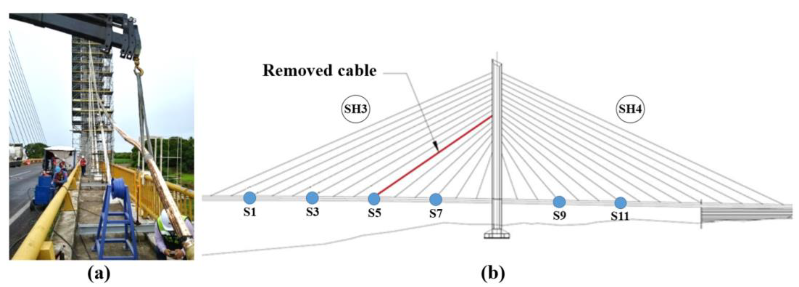
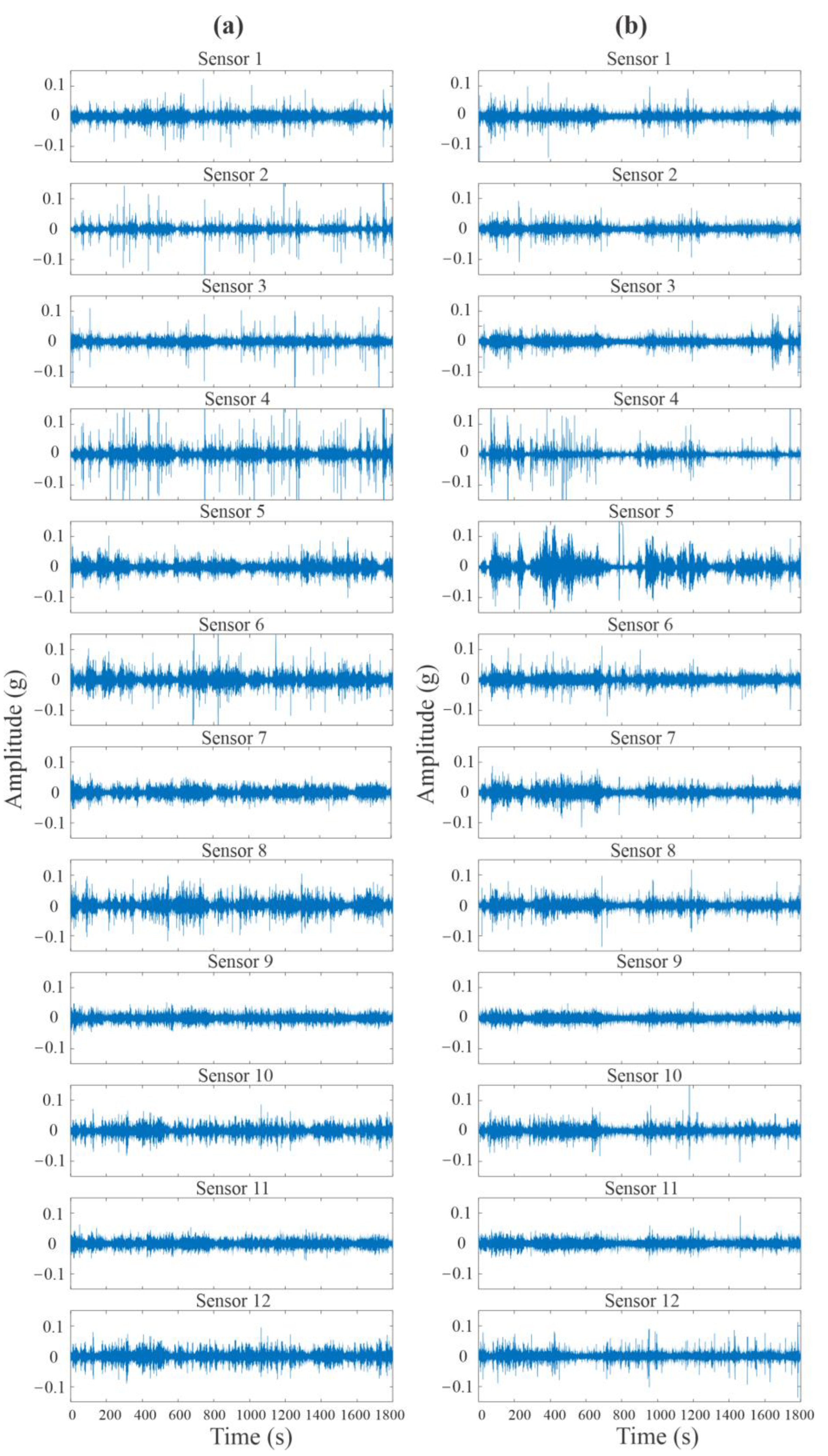
Following the experimental procedure described in Section 2.2, as well as the damage detection methodology presented in Section 3.3, the entropy–CWT diagram is obtained for the analyzed damaged case (removed cable) and compared with the healthy scenario. Thus, the average SEI for the CWT coefficients considering all measurement points (sensors S1–S12 in Figure 4) is plotted in just a few seconds. In order to provide some examples of the type of experimental signals acquired/analyzed, in Figure 27, the experimental time-domain signals acquired from the RPB considering the total time duration of 1800 s for each sensor of the two scenarios (healthy and damaged RPB) are shown, whereas, in Figure 28, the corresponding entropy–CWT diagram for the damaged case is presented.

As can be observed in Figure 28, the useful scale range, used to conduct the analysis and identify damage, is similar to the numerical cases. Therefore, for this experimental case, the scale range considered is from 200 onwards (200 to 1000).

Subsequently, all the signals for the healthy and damaged cases are filtered and extended, taking into account the same type of filter and the parameters used for the numerical cases. After that, the average CWT coefficients for the scale range from 200 to 1000 are calculated for each of the 30 segments of 1 min for each sensor of the healthy bridge (12 sensors) and the damaged bridge (12 sensors). Lastly, the maximum value of the average CWT coefficients for the 720 files are registered; finally, for each sensor of each condition (healthy and damaged), a unique value of the maximum CWT coefficient is obtained considering the average of the 30 respective maximum values of each sensor/condition. 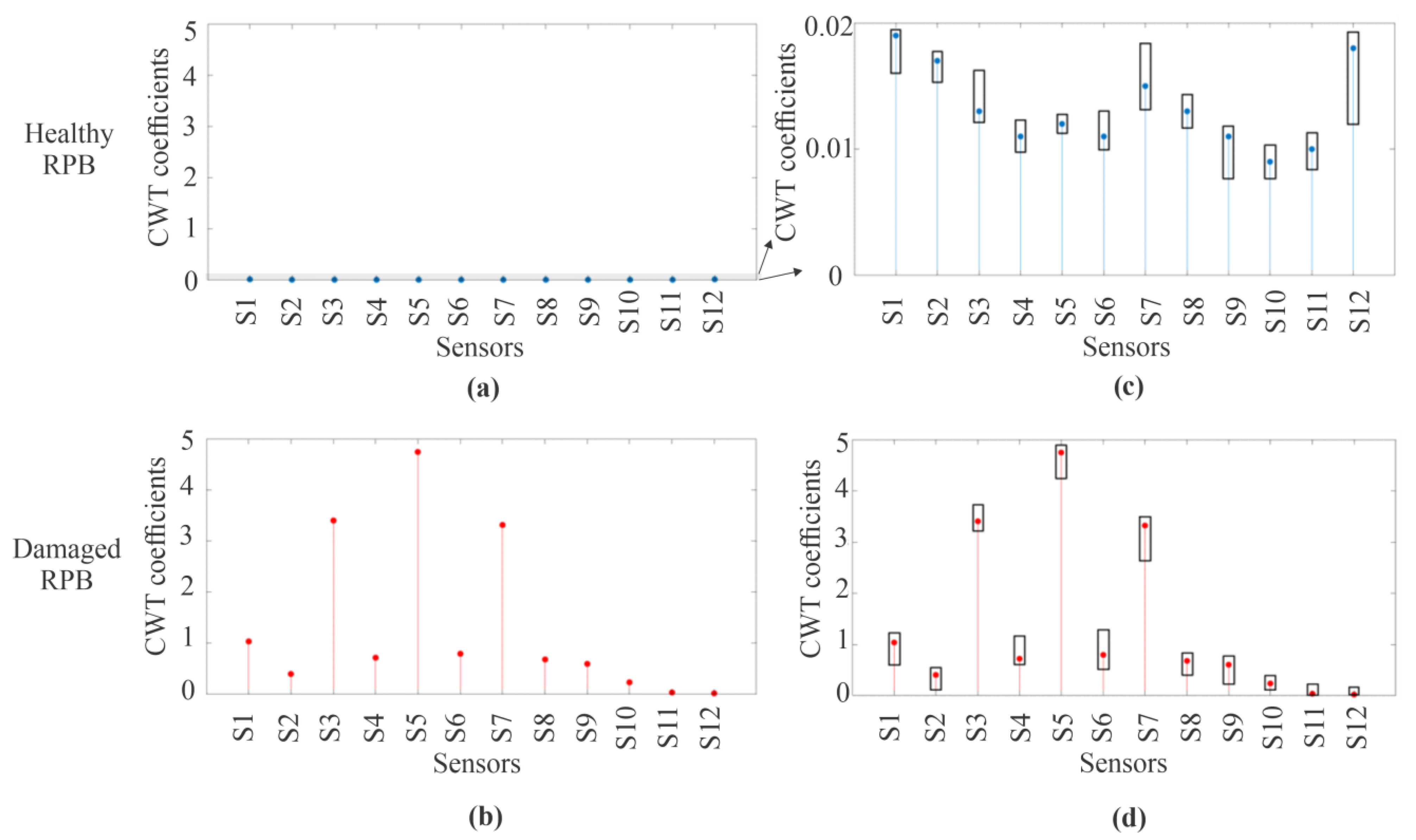These final maximum average values are indicated in Figure 29 thought solid circles, while the corresponding minimum and maximum values obtained for the respective 30 tests of each case are indicated with horizontal solid lines.

Thus, in the corresponding results presented in Figure 29, it is possible to observe that, for the damage case, the maximum value of the average CWT coefficients (solid circle) corresponds clearly with sensor S5, whose position on the bridge deck is the same as that of the lower anchoring of the removed cable. On the other hand, if the respective results of the healthy case are compared with the ones of the damaged cases, it is evident that the maximum values of the average CWT coefficients are always higher for the damaged cases. Moreover, there is also a clear tendency that, even when considering the minimum and maximum values obtained for each set of 30 tests, the CWT coefficients are much higher for the damaged RPB, and particularly for the sensor located in the position of damage (S5).

Regardless of whether the experimental validation of a controlled test was not possible with the same conditions as the numerical simulations (just one vehicle crossing the bridge with a specific weight and a specific constant speed) or, conversely, whether the transit was random, the experimental results show good agreement with the numerical results, and they were obtained as fast as the numerical results were, thus validating and highlighting the advantages of this new method, focused mainly on the good precision, low computational burden, efficient obtaining of results, and low cost.

Even though promising results have been achieved in this specific scenario, further research is necessary in order to enhance the robustness of the proposed method. In this regard, it is important to explore other case studies that address the following scenarios: (i) sensor placement does not align with or is far away from the damage zone, (ii) varying quantities of sensors are to be employed, and (iii) a wider range of damages, such as additional cable removal, corrosion, loosened bolts, among others, are present. This calibration of the proposal under these circumstances will allow for the investigation of diverse scenarios where sensor triggering may occur. Currently, the performance of the proposed method can be compromised in these scenarios, as its accuracy in both damage detection and localization heavily relies on the quantity and positioning of the sensors. For instance, a limited number of sensors diminishes the system’s capability of detecting vibrations associated with damage across the entire bridge, and reduces the resolution for determining or identifying the damage location, especially in the context of a large bridge, such as the one analyzed in this work.

Hence, real-world experiments, considering other conditions (additional types of damage and alternative sensor orientations or directions), are essential for validating and calibrating structural health monitoring strategies, but conducting analyses on actual bridges under both healthy and damaged conditions poses significant challenges in terms of human resources, infrastructure, and financial constraints. In addition to the previously mentioned issues, the obtaining of the vibrational signature of a new bridge, through considering all available vibration sensors and their locations, will play a crucial role in assessing the accuracy and sensitivity of the proposed method for detecting and locating various types of damage. This effort will be always supported by modeling and computational simulations.

6. Conclusions

This article presents, in detail, the development of the EWM, which is an improved version of the WEAM presented in [1], and whose main objective is to detect and locate damage in highway bridges more efficiently. In particular, the EWM eliminates a large number of steps from the WEAM, providing a simpler, faster, and more accurate method of damage identification.

To give way to this new method, an algorithm based on the Shannon entropy was implemented, which allows us to know, from the vibration signals acquired on a bridge, the level of chaos produced by the respective CWT coefficients of the signals, and what CWT scale they correspond to. In a similar way to the entropy–CWT diagram, three zones are established for different CWT scale ranges according to the level of chaos of the CWT coefficients and the causes that generate those levels of chaos (effects of natural frequencies, edge effects, and effects of structural damage).

In this way, the entropy–CWT diagram allows for the defining of the useful CWT scale range in order to identify damage by averaging the CWT coefficients, and is obtained in a few seconds (less than 7 s for each measurement point analyzed in this article). This is dissimilar to the WEAM, which, for the same purpose of establishing the useful CWT scale range, requires the generation of colored 3D CWT diagrams that require a high computational load.

For validation, the EWM was applied in a finite element model of the RPB, considering the healthy case and different damage scenarios. The results indicate that the EWM is capable of identifying the diverse damage conditions successfully, detecting damage clearly, with localization precision between 98.76% and 99.97% and with results obtained quickly (around 51 s).

Therefore, the numerical results of the application of the EWM are promising, since, when compared to the WEAM, the precision in locating the damage is further increased, which was already very good with the WEAM (increase of approximately 0.11%). Above all, the disadvantages of the WEAM related to the number of stages required to apply the method are eliminated (going from 11 to 7 stages), thus reducing the computing time by 5.67 times.

Furthermore, the experimental validation shows that the EWM was able to identify damage in the real-life RPB (removed cable), even when using random transit, thus reinforcing the advantages of this method. In future works, this method will be applied considering diverse severities of damage in different cables of the numerical model, as well as in the real real-life RPB with removed cables in different positions.

References

1. Machorro-Lopez, J.M.; Amezquita-Sanchez, J.P.; Valtierra-Rodriguez, M.; Carrion-Viramontes, F.J.; Quintana-Rodriguez, J.A.; Valenzuela-Delgado, J.I. Wavelet Energy Accumulation Method Applied on the Rio Papaloapan Bridge for Damage Identification. Mathematics 2021, 9, 422. [Google Scholar] [CrossRef]
2. Prus, P.; Sikora, M. The Impact of Transport Infrastructure on the Sustainable Development of the Region—Case Study. Agriculture 2021, 11, 279. [Google Scholar] [CrossRef]
3. Sharma, N.; Nocera, F.; Gardoni, P. Classification and Mathematical Modeling of Infrastructure Interdependencies. Sustain. Resilient Infrastruct. 2020, 6, 4–25. [Google Scholar] [CrossRef]
4. Robert, O.-K.; Tam, V.; Ma, M.; Mashiri, F. Critical Review of the Threats Affecting the Building of Critical Infrastructure Resilience. Int. J. Disaster Risk Reduct. 2021, 60, 102316. [Google Scholar] [CrossRef]
5. Alshahrani, A.; Alaboud, N.; Leje, M.I.; Karban, A.; Altowerqi, Z. Rating the Significance of the Factors Influencing Shortage of Skilled Labours for Sustainable Construction: A Perception of Makkah Construction Practitioner. J. Umm Al-Qura Univ. Eng. Archit. 2023, 14, 13–25. [Google Scholar] [CrossRef]
6. Boakye, J.; Guidotti, R.; Gardoni, P.; Murphy, C. The Role of Transportation Infrastructure on the Impact of Natural Hazards on Communities. Reliab. Eng. Syst. Saf. 2022, 219, 108184. [Google Scholar] [CrossRef]
7. Estes, A.C.; Frangopol, D.M. Bridge Lifetime System Reliability under Multiple Limit States. J. Bridge Eng. 2001, 6, 523–528. [Google Scholar] [CrossRef]
8. Greco, F.; Lonetti, P.; Zinno, R. An Analytical Delamination Model for Laminated Plates Including Bridging Effects. Int. J. Solids Struct. 2002, 39, 2435–2463. [Google Scholar] [CrossRef]
9. Ford, K.M.; Arman, M.H.R.; Labi, S.; Sinha, K.C.; Thompson, P.D.; Shirole, A.M.; Li, Z. Estimating Life Expectancies of Highway Assets, Volume 2: Final Report; Transportation Research Board: Washington, DC, USA, 2012; ISBN 978-0-309-21408-7. [Google Scholar]
10. Milillo, P.; Giardina, G.; Perissin, D.; Milillo, G.; Coletta, A.; Terranova, C. Pre-Collapse Space Geodetic Observations of Critical Infrastructure: The Morandi Bridge, Genoa, Italy. Remote Sens. 2019, 11, 1403. [Google Scholar] [CrossRef]
11. Sohn, H.; Farrar, C.R.; Hemez, F.M.; Czarnecki, J.J. A Review of Structural Health Review of Structural Health Monitoring Literature 1996–2001; Los Alamos National Laboratory (LANL): Los Alamos, NM, USA, 2002.
12. Haritos, N.; Owen, J.S. The Use of Vibration Data for Damage Detection in Bridges: A Comparison of System Identification and Pattern Recognition Approaches. Struct. Health Monit. 2004, 3, 141–163. [Google Scholar] [CrossRef]
13. Carmo, J.S.A.D. The Hintze Ribeiro Bridge Collapse and the Lessons Learned. In River Basin Management—Sustainability Issues and Planning Strategies; IntechOpen: London, UK, 2021; ISBN 978-1-83968-131-8. [Google Scholar]
14. LeRose, C. The Collapse of the Silver Bridge; West Virginia Historical Society Quarterly: Charleston, WV, USA, 2001. [Google Scholar]
15. Davey, M.; Wald, M.L. Potential Flaw Is Found in Design of Fallen Bridge. The New York Times, 2007. [Google Scholar]
16. Mattioli, G. What Caused the Genoa Bridge Collapse—And the End of an Italian National Myth? The Guardian, 2019. [Google Scholar]
17. Penn, A. The Deadliest Bridge Collapses in the US in the Last 50 Years. Available online: https://www.cnn.com/2018/03/15/us/bridge-collapse-history-trnd/index.html (accessed on 26 February 2024).
18. Lazo, C.; Gallardo, P.; Céspedes, S. A Bridge Structural Health Monitoring System Supported by the Internet of Things. In Proceedings of the IEEE Colombian Conference on Communication and Computing (IEEE COLCOM 2015), Popayan, Colombia, 13–15 May 2015; pp. 1–6. [Google Scholar]
19. Wijetunge, S.; Gunawardana, U.; Liyanapathirana, R. Wireless Sensor Networks for Structural Health Monitoring: Considerations for Communication Protocol Design. In Proceedings of the 2010 17th International Conference on Telecommunications, Doha, Qatar, 4–7 April 2010; pp. 694–699. [Google Scholar]
20. Hu, X.; Wang, B.; Ji, H. A Wireless Sensor Network-Based Structural Health Monitoring System for Highway Bridges. Comput. -Aided Civ. Infrastruct. Eng. 2013, 28, 193–209. [Google Scholar] [CrossRef]
21. Dai, Z.; Wang, S.; Yan, Z. BSHM-WSN: A Wireless Sensor Network for Bridge Structure Health Monitoring. In Proceedings of the 2012 Proceedings of International Conference on Modelling, Identification and Control, Wuhan, China, 24–26 June 2012; pp. 708–712. [Google Scholar]
22. Modares, M.; Waksmanski, N. Overview of Structural Health Monitoring for Steel Bridges. Pract. Period. Struct. Des. Constr. 2013, 18, 187–191. [Google Scholar] [CrossRef]
23. Farrar, C.R.; Worden, K. An Introduction to Structural Health Monitoring. Philos. Trans. A Math Phys. Eng. Sci. 2007, 365, 303–315. [Google Scholar] [CrossRef] [PubMed]
24. Farrar, C.R.; Lieven, N.A.J. Damage Prognosis: The Future of Structural Health Monitoring. Philos. Trans. R. Soc. A Math. Phys. Eng. Sci. 2006, 365, 623–632. [Google Scholar] [CrossRef]
25. Kong, X.; Cai, C.-S.; Hu, J. The State-of-the-Art on Framework of Vibration-Based Structural Damage Identification for Decision Making. Appl. Sci. 2017, 7, 497. [Google Scholar] [CrossRef]
26. Bert, C.W. Relationship Between Fundamental Natural Frequency And Maximum Static Deflection For Various Linear Vibratory Systems. J. Sound Vib. 1993, 162, 547–557. [Google Scholar] [CrossRef]
27. Abdel wahab, M.M.; De roeck, G. Damage Detection in Bridges using Modal Curvatures: Application to a Real Damage Scenario. J. Sound Vib. 1999, 226, 217–235. [Google Scholar] [CrossRef]
28. Salawu, O.S. Detection of Structural Damage through Changes in Frequency: A Review. Eng. Struct. 1997, 19, 718–723. [Google Scholar] [CrossRef]
29. Pandey, A.K.; Biswas, M.; Samman, M.M. Damage Detection from Changes in Curvature Mode Shapes. J. Sound Vib. 1991, 145, 321–332. [Google Scholar] [CrossRef]
30. Zimmerman, D.C.; Kaouk, M. Structural Damage Detection Using a Minimum Rank Update Theory. J. Vib. Acoust. 1994, 116, 222–231. [Google Scholar] [CrossRef]
31. Avci, O.; Abdeljaber, O.; Kiranyaz, S.; Hussein, M.; Gabbouj, M.; Inman, D.J. A Review of Vibration-Based Damage Detection in Civil Structures: From Traditional Methods to Machine Learning and Deep Learning Applications. Mech. Syst. Signal Process. 2021, 147, 107077. [Google Scholar] [CrossRef]
32. Liew, K.M.; Wang, Q. Application of Wavelet Theory for Crack Identification in Structures. J. Eng. Mech. 1998, 124, 152–157. [Google Scholar] [CrossRef]
33. Hou, Z.; Noori, M.; Amand, R.S. Wavelet-Based Approach for Structural Damage Detection. J. Eng. Mech. 2000, 126, 677–683. [Google Scholar] [CrossRef]
34. Douka, E.; Loutridis, S.; Trochidis, A. Crack Identification in Beams Using Wavelet Analysis. Int. J. Solids Struct. 2003, 40, 3557–3569. [Google Scholar] [CrossRef]
35. Machorro-López, J.M.; Bellino, A.; Marchesiello, S.; Garibaldi, L. Damage Detection for Beams Subject to Moving Loads Based on Wavelet Transforms. In Proceedings of the 11th International Conference on Computational Structures Technology, Dubrovnik, Croatia, 4–7 September 2012; p. 79. [Google Scholar]
36. Xu, Y.L.; Chen, J. Structural Damage Detection Using Empirical Mode Decomposition: Experimental Investigation. J. Eng. Mech. 2004, 130, 1279–1288. [Google Scholar] [CrossRef]
37. Chen, J. Application of Empirical Mode Decomposition in Structural Health Monitoring: Some Experience. Adv. Adapt. Data Anal. 2009, 01, 601–621. [Google Scholar] [CrossRef]
38. Dong, Y.; Li, Y.; Lai, M. Structural Damage Detection Using Empirical-Mode Decomposition and Vector Autoregressive Moving Average Model. Soil Dyn. Earthq. Eng. 2010, 30, 133–145. [Google Scholar] [CrossRef]
39. Omenzetter, P.; Brownjohn, J.M.W. Application of Time Series Analysis for Bridge Monitoring. Smart Mater. Struct. 2006, 15, 129. [Google Scholar] [CrossRef]
40. Kopsaftopoulos, F.P.; Fassois, S.D. Vibration Based Health Monitoring for a Lightweight Truss Structure: Experimental Assessment of Several Statistical Time Series Methods. Mech. Syst. Signal Process. 2010, 24, 1977–1997. [Google Scholar] [CrossRef]
41. Mei, Q.; Gül, M. A Fixed-Order Time Series Model for Damage Detection and Localization. J. Civ. Struct. Health Monit. 2016, 6, 763–777. [Google Scholar] [CrossRef]
42. Jiang, X.; Adeli, H. Pseudospectra, MUSIC, and Dynamic Wavelet Neural Network for Damage Detection of Highrise Buildings. Int. J. Numer. Methods Eng. 2007, 71, 606–629. [Google Scholar] [CrossRef]
43. Perez-Ramirez, C.A.; Machorro-Lopez, J.M.; Valtierra-Rodriguez, M.; Amezquita-Sanchez, J.P.; Garcia-Perez, A.; Camarena-Martinez, D.; Romero-Troncoso, R.d.J. Location of Multiple Damage Types in a Truss-Type Structure Using Multiple Signal Classification Method and Vibration Signals. Mathematics 2020, 8, 932. [Google Scholar] [CrossRef]
44. Machorro-Lopez, J.M.; Valtierra-Rodriguez, M.; Amezquita-Sanchez, J.P.; Carrion-Viramontes, F.J.; Quintana-Rodriguez, J.A. A Shannon Entropy-Based Methodology to Detect and Locate Cables Loss in a Cable-Stayed Bridge. Int. J. Appl. Mech. 2021, 13, 2150063. [Google Scholar] [CrossRef]
45. Moreno-Gomez, A.; Amezquita-Sanchez, J.P.; Valtierra-Rodriguez, M.; Perez-Ramirez, C.A.; Dominguez-Gonzalez, A.; Chavez-Alegria, O. EMD-Shannon Entropy-Based Methodology to Detect Incipient Damages in a Truss Structure. Appl. Sci. 2018, 8, 2068. [Google Scholar] [CrossRef]
46. Xie, Z.K.; Liu, G.H.; Zhang, Z.H. Damage Detection of Concrete Structure Based on Approximate Entropy. Appl. Mech. Mater. 2012, 226–228, 920–925. [Google Scholar] [CrossRef]
47. Lin, T.-K.; Laínez, A.G. Entropy-Based Structural Health Monitoring System for Damage Detection in Multi-Bay Three-Dimensional Structures. Entropy 2018, 20, 49. [Google Scholar] [CrossRef] [PubMed]
48. Khodabandehlou, H.; Pekcan, G.; Fadali, M.S. Vibration-Based Structural Condition Assessment Using Convolution Neural Networks. Struct. Control Health Monit. 2019, 26, e2308. [Google Scholar] [CrossRef]
49. Dorafshan, S.; Azari, H. Evaluation of Bridge Decks with Overlays Using Impact Echo, a Deep Learning Approach. Autom. Constr. 2020, 113, 103133. [Google Scholar] [CrossRef]
50. Gao, Y.; Mosalam, K.M. Deep Transfer Learning for Image-Based Structural Damage Recognition. Comput.-Aided Civ. Infrastruct. Eng. 2018, 33, 748–768. [Google Scholar] [CrossRef]
51. Lei, G.; Liao, Q.; Patil, S. A Fractal Model for Relative Permeability in Fractures under Stress Dependence. Fractals 2019, 27, 1950092. [Google Scholar] [CrossRef]
52. Moreno-Gomez, A.; Machorro-Lopez, J.M.; Amezquita-Sanchez, J.P.; Perez-Ramirez, C.A.; Valtierra-Rodriguez, M.; Dominguez-Gonzalez, A. Fractal Dimension Analysis for Assessing the Health Condition of a Truss Structure Using Vibration Signals. Fractals 2020, 28, 2050127. [Google Scholar] [CrossRef]
53. Candès, E.J.; Li, X.; Ma, Y.; Wright, J. Robust Principal Component Analysis? JACM 2011, 58, 1–37. [Google Scholar] [CrossRef]
54. Bellino, A.; Machorro-Lopez, J.M.; Marchesiello, S.; Garibaldi, L. Damage Detection in Structures under Variations of Temperature and Clamping Conditions; IRIS: Turin, Italy, 2012. [Google Scholar]
55. Machorro-Lopez, J.M.; Bellino, A.; Garibaldi, L.; Adams, D.E. PCA-Based Techniques for Detecting Cracked Rotating Shafts Including the Effects of Temperature Variations. Eng. Mater. Sci. 2011, 1, 1–8. [Google Scholar]
56. Mujica, L.E.; Ruiz, M.; Pozo, F.; Rodellar, J.; Güemes, A. A Structural Damage Detection Indicator Based on Principal Component Analysis and Statistical Hypothesis Testing. Smart Mater. Struct. 2013, 23, 025014. [Google Scholar] [CrossRef]
57. Shannon, C.E. A Mathematical Theory of Communication. Bell Syst. Tech. J. 1948, 27, 379–423. [Google Scholar] [CrossRef]
58. Sethna, J.P. Entropy, Order Parameters, and Complexity; Oxford University Press: Oxford, UK, 2006. [Google Scholar]
59. Perez-Ramirez, C.A.; Amezquita-Sanchez, J.P.; Valtierra-Rodriguez, M.; Adeli, H.; Dominguez-Gonzalez, A.; Romero-Troncoso, R.J. Recurrent Neural Network Model with Bayesian Training and Mutual Information for Response Prediction of Large Buildings. Eng. Struct. 2019, 178, 603–615. [Google Scholar] [CrossRef]
60. Mousavi, M.; Holloway, D.; Olivier, J.C.; Alavi, A.H.; Gandomi, A.H. A Shannon Entropy Approach for Structural Damage Identification Based on Self-Powered Sensor Data. Eng. Struct. 2019, 200, 109619. [Google Scholar] [CrossRef]
61. Shapiro, S.S.; Zahedi, H. Bernoulli Trials and Discrete Distributions. J. Qual. Technol. 1990, 22, 193–205. [Google Scholar] [CrossRef]
62. Rucka, M.; Wilde, K. Crack Identification Using Wavelets on Experimental Static Deflection Profiles. Eng. Struct. 2006, 28, 279–288. [Google Scholar] [CrossRef]
63. Liu, C.-L. A Tutorial of the Wavelet Transform; NTUEE: Taipei City, Taiwan, 2010. [Google Scholar]
64. Winkler, T. How Realistic Is Artificially Added Noise? In Proceedings of the Twelfth Annual Conference of the International Speech Communication Association, Florence, Italy, 27–31 August 2011.
Figure 1. Pictures of the RPB.
Applsci 14 03298 g001
Figure 2. Drawing of the RPB.
Applsci 14 03298 g002
Figure 3. FEM model of the RPB in ANSYS©.
Applsci 14 03298 g003
Figure 4. (a) Accelerometer installed on the RPB deck, and (b) the location of the sensors (S1–S12) used to acquire the dynamic responses of the RPB.
Applsci 14 03298 g004
Figure 5. Removed stay-cable, generating the damaged condition on the RPB (red line): (a) real-life condition and (b) schematic representation.
Applsci 14 03298 g005
Figure 6. Representation of the SEI.
Applsci 14 03298 g006
Figure 7. Representation of the CWT.
Applsci 14 03298 g007
Figure 8. Schematic diagram of the EWM and WEAM methods.
Applsci 14 03298 g008
Figure 9. CWT coefficients for each scale value from 1 to 1000, corresponding to the scenario with damage at 25% of L and measuring at 25% of L.
Applsci 14 03298 g009
Figure 10. CWT coefficients for the scale range from 1 to 1000 with increments of 50, corresponding to the scenario with damage at 25% of L and measuring at 25% of L.
Applsci 14 03298 g010
Figure 11. Entropy–CWT diagram, plotting the average SEI for the CWT coefficients considering all measurement points (25%, 50%, and 75% of L) for the case of a bridge with a deck damaged at 0.25 L and a scale range from 1 to 1000.
Applsci 14 03298 g011
Figure 12. CWT diagrams from original acceleration signals for the case of a bridge with a damaged deck at 0.25 L applying the WEAM. Three different measuring positions (from top to bottom: (a) 0.25 L, (b) 0.50 L, and (c) 0.75 L [1].
Applsci 14 03298 g012
Figure 13. Average CWT coefficients for the scale range from 1 to 100, corresponding to the scenario with damage at 25% of L and measuring at 25% of L.
Applsci 14 03298 g013
Figure 14. Average CWT coefficients for the scale range from 101 to 181, corresponding to the scenario with damage at 25% of L and measuring at 25% of L.
Applsci 14 03298 g014
Figure 15. Average CWT coefficients for the scale range from 181 to 500, corresponding to the scenario with damage at 25% of L and measuring at 25% of L.
Applsci 14 03298 g015
Figure 16. Average CWT coefficients for the scale range from 181 to 1000, corresponding to the scenario with damage at 25% of L and measuring at 25% of L.
Applsci 14 03298 g016
Figure 17. Average CWT coefficients for the scale range from 181 to 1000 from the respective average of 3 measurement points (25%, 50%, and 75% of L), corresponding to the scenarios of the healthy bridge and the bridge with damage at 25% of L.
Applsci 14 03298 g017
Figure 18. Average CWT coefficients for the scale range from 181 to 1000 from the respective average of 3 measurement points (25%, 50%, and 75% of L) with signals previously extended to eliminate edge effects. Scenarios shown: healthy bridge and bridge with damage at 25% L.
Applsci 14 03298 g018
Figure 19. Average CWT coefficients for the scale range from 181 to 1000 from the respective average of 3 measurement points (25%, 50%, and 75% of L) with noisy signals (15% Gaussian noise), extended to remove edge effects. Scenarios shown: healthy bridge and bridge with damage at 25% L.
Applsci 14 03298 g019
Figure 20. Average CWT coefficients for the scale range from 181 to 1000 from the respective average of 3 measurement points (25%, 50%, and 75% of L) with signals filtered from noisy signals (15% Gaussian noise), extended to remove edge effects. Scenarios shown: healthy bridge and bridge with intermediate severity damage (30% intensity) at 25% L.
Applsci 14 03298 g020
Figure 21. CWT coefficients for the scale value of 300, corresponding to the scenario with damage at 25% of L and measuring at 25% of L. Edge effects without being removed.
Applsci 14 03298 g021
Figure 22. CWT coefficients for the scale value of 300, corresponding to the scenario with damage at 25% of L and measuring at 25% of L. Edge effects eliminated via signal extension.
Applsci 14 03298 g022
Figure 23. Average CWT coefficients for the scale range from 181 to 1000 from the respective average of 3 measurement points (25%, 50%, and 75% of L) with signals filtered from noisy signals (15% Gaussian noise), extended to remove edge effects. Scenarios shown: healthy bridge and bridge with low severity damage (10% intensity) at 50% L.
Applsci 14 03298 g023
Figure 24. Average CWT coefficients for the scale range from 181 to 1000 from the respective average of 3 measurement points (25%, 50%, and 75% of L) with signals filtered from noisy signals (15% Gaussian noise), extended to remove edge effects. Scenarios shown: healthy bridge and bridge with high severity damage (50% intensity) at 75% L.
Applsci 14 03298 g024
Figure 25. CWT coefficients for the scale value of 300, corresponding to the scenario with damage at 75% of L and measuring at 25% of L. Edge effects eliminated by signal extension.
Applsci 14 03298 g025
Figure 26. Average CWT coefficients for the scale range from 181 to 1000 from the respective average of 3 measurement points (25%, 50%, and 75% of L) with signals filtered from noisy signals (15% Gaussian noise), extended to remove edge effects. Scenarios shown: healthy bridge and bridge with intermediate severity damage (30% intensity) at 75% L.
Applsci 14 03298 g026
Figure 27. Experimental time-domain signals acquired from the real-life RPB, considering the total time duration of 1800 s for each sensor (Sensor 1–Sensor 12) of the following two scenarios: (a) healthy RPB, and (b) damaged RPB with a removed cable.
Applsci 14 03298 g027
Figure 28. Entropy–CWT diagram, plotting the average SEI for the CWT coefficients considering all measurement points (sensors S1–S12 in Figure 4) for the experimental case of the real-life RPB with a removed cable and a scale range from 1 to 1000. The below plot focuses on the above plot, showing the entropy increments resulting from damage.
Applsci 14 03298 g028
Figure 29. Values of maximum CWT coefficient considering the average of the 30 respective maximum values of each sensor/condition with a scale range from 200 to 1000 (solid circles) for (a,c) healthy RPB and (b,d) damaged RPB with a removed cable. For the first two plots (a,b), the same vertical scale is considered for identifying damage quickly. Fore the last two plots (c,d), the vertical scale is auto-adjusted for both scenarios (healthy and damage) to visualize the corresponding minimum and maximum values obtained for the respective 30 tests of each case (horizontal solid lines).
Applsci 14 03298 g029
Disclaimer/Publisher’s Note: The statements, opinions and data contained in all publications are solely those of the individual author(s) and contributor(s) and not of MDPI and/or the editor(s). MDPI and/or the editor(s) disclaim responsibility for any injury to people or property resulting from any ideas, methods, instructions or products referred to in the content.