Abstract
Leakage in water supply pipelines remains a significant challenge. It leads to resource and economic waste. Researchers have developed several leak detection methods, including the use of embedded sensors and pressure prediction. The former approach involves pre-installing detectors inside pipelines to detect leaks. This method allows for the precise localization of leak points. The stability is compromised because of the wireless signal strength. The latter approach, which relies on pressure measurements to predict leak events, does not achieve precise leak point localization. To address these challenges, in this paper, a coherent optical time-domain reflectometry (φ-OTDR) system is employed to capture vibration signal phase information. Subsequently, two pre-trained neural network models based on CNN and Resnet18 are responsible for processing this information to accurately identify vibration events. In an experimental setup simulating water pipelines, phase information from both leaking and non-leaking pipe segments is collected. Using this dataset, classical CNN and ResNet18 models are trained, achieving accuracy rates of 99.7% and 99.5%, respectively. The multi-leakage point experiment results indicate that the Resnet18 model has better generalization compared to the CNN model. The proposed solution enables long-distance water-pipeline precise leak point localization and accurate vibration event identification.
1. Introduction
Water is an indispensable and important substance for the survival of human beings and all living things and is an irreplaceable and extremely valuable natural resource for industrial and agricultural production, economic development, and environmental improvement. However, many countries in the world are facing the problem of water shortage. Take China as an example. Although China is a water-rich nation, it also suffers from severe water shortages on a per capita basis. According to statistics, China’s per capita water resources comprise less than 2200 cubic meters, less than one-third of the world’s per capita water resources [1]. Among the 660 cities in China, approximately 400 cities are short of water. With the development and construction of the country, the water usage rates of various cities are increasing year by year, and the lengths of urban water supply pipelines are also increasing. Consequently, society places higher demands on the quality of urban water supply networks, which is crucial for ensuring stable development [2,3,4]. However, in terms of the construction of China’s overall municipal water supply network, many places still have the problem of pipeline leakage, which causes residents to be forced to cut off water and even causes accidents such as road collapse, resulting in the wastage of water resources and economic damage. The primary problem for reducing the leakage rate in a city concerns how to accurately know that the water supply pipeline has leaked, and it is necessary to accurately locate the location of the leakage point so as to be able to quickly repair and reduce the wastage of resources. Therefore, it is necessary to develop a system that can monitor the precise location of leaks in real time when leaks occur in the water supply network.
Mainstream pipeline leak detection technologies include the magnetic flux leakage (MFL) detection method, pipeline robot inspection method, water pressure prediction method, and Distributed Acoustic Sensing (DAS) method. The MFL detection method is a commonly used method for pipeline inspection [5]. The principle behind MFL detection involves fully magnetizing the pipeline, causing magnetic field lines to deform at the locations of defects. These deformed lines flow out from a defect and then return to the interior of the pipeline. Sensors carried by the inspection system detect and store this information, allowing the accurate localization of pipeline leaks. While this approach offers high precision in leak localization, it is limited to ferromagnetic pipelines. The pipeline robot inspection method uses robots within the pipelines to monitor their condition. Simultaneously, a wireless sensor network is installed on the ground to receive data [6,7]. However, this approach faces several challenges. Firstly, in practical scenarios, pipes are often buried deep underground, hindering wireless signal transmission. Additionally, there is a risk of robots becoming stuck within the pipes, leading to blockages. The water pressure prediction method uses water pressure values to predict water leakage. Mashford et al. employed Support Vector Machines (SVMs) to classify data from the EPANET hydraulic modeling system, resulting in improved leak prediction [8]. Leu et al. further enhanced leak prediction accuracy through Bayesian learning processes [9]. The proposed solution suffers from a limitation: it cannot provide precise information about the exact locations of leaks. Distributed Acoustic Sensing (DAS) tackles water leakage detection by capturing vibration signals associated with leak locations. DAS is widely applicable to both ferromagnetic and non-ferromagnetic pipelines, offering the precise localization of vibration signals. In 2015, Huijuan Wu et al. successfully detected water pipe leaks by deploying communication optical fibers along the inner walls of pipelines, achieving leak detection when under conditions where the aperture exceeded 4 mm and internal pressure exceeded 0.2 MPa [10]. In 2022, Shichong Fu et al. utilized DAS systems to achieve meter-level spatial resolution for pinpointing gas pipeline leak points. Their study also explored how leak hole size and leak direction impact the spectral characteristics of leak signals [11]. However, none of the aforementioned works in the literature delved into the discussion of leak event recognition accuracy.
In practice, while achieving leak localization is feasible, false positives and false negatives remain significant challenges for DAS systems. Initially, researchers relied on threshold settings for accurate vibration event identification. In 2014, Zhu et al. set a level threshold to determine the event category [12]. In 2018, Jiang et al. used the amplitude of the vibration signal as the basis for judging whether there was a vibration event by setting a threshold and achieved a recognition accuracy of 95.57% for a specific “instantaneous destructive disturbance” in a laboratory environment [13]. However, pattern recognition is only performed through thresholds, and its recognition accuracy and stability are poor in practical application scenarios. It is difficult to ensure the stability of the signal-to-noise ratio of the received signal due to the attenuation of the signal in the process of long-distance transmission, coupled with the influence of coherent fading and polarization fading, which leads to the inaccuracy of the frequency characteristics demodulated. The disturbance signals on the optical fiber are intricately intertwined, and even the vibration signals that need to be detected are dynamically changing, which further leads to a reduction in the recognition accuracy of the system.
Pattern recognition through machine learning is a popular solution. By analyzing existing data and selecting appropriate algorithms, a model can be built and continuously optimized, and finally, various events can be identified quickly and accurately. The concept of machine learning was first proposed by the American computer scientist Arthur Samuel in 1959 as a branch of artificial intelligence (AI) and computer science that focuses on the use of data and algorithms to enable AI to mimic human learning methods and gradually improve its recognition accuracy [14]. In 1998, LeCun et al. proposed a model architecture for convolutional neural networks (CNNs) and applied them to the task of handwriting number recognition [15]. The LeNet-5 model proposed by LeCun achieved excellent performance on the MNIST dataset, marking the birth of deep learning and achieving more complex feature extraction. In 2015, Kaiming He et al. proposed the ResNet18 neural network, which solves the gradient vanishing problem that may occur when the number of layers in traditional CNN networks increases [16]. The emergence of these models provides a strong guarantee for the accurate realization of pattern recognition.
In this paper, a coherent φ-OTDR system is employed to capture vibration signal phase information and a pre-trained neural network model is responsible for processing this information to accurately identify leakage events and locations. The proposed method is evaluated in a simulated water pipelines setup. Phase information from both leaking and non-leaking pipe segments is collected to create separate datasets for training different models: CNN and ResNet18. During practical testing, the test accuracy values of the CNN model and ResNet18 model achieve 99.7% and 99.5%, respectively. What is more, in the multi-leakage point detection experiment, the ResNet18 model performs better, which indicates that Resnet18 has better generalization ability compared to the CNN model.
2. Sensing Principle of φ-OTDR
Optical pulses propagate through optical fibers, and due to the uneven refractive index distribution of fibers, Rayleigh scattering occurs [17]. Some of the scattered light will be back-guided towards the input end of the fiber and will be detected with a delay proportional to the distance of the diffusing point, which is called optical time-domain reflection.
There is a relationship between the length d of the optical fiber link through which the incident light passes and the time delay τ between the incident light and the scattered light:
Here, c represents the speed of light in a vacuum and n denotes the effective refractive index of the fundamental mode of SMF.
The system’s positioning accuracy, denoted as z, primarily depends on the pulse width, represented by T; then, the spatial resolution z can be written as follows:
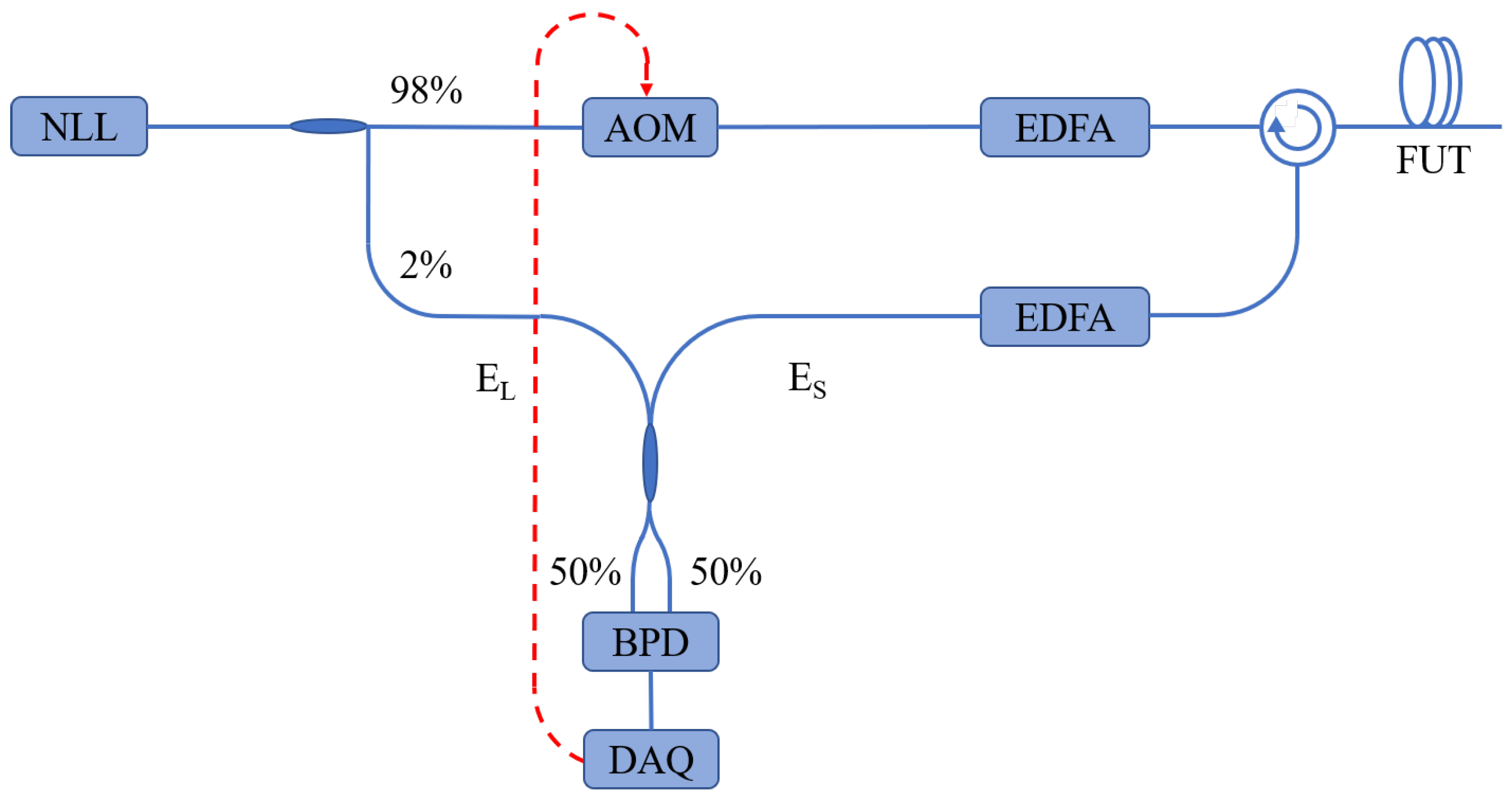
When the refractive index of fiber section at the corresponding location undergoes slight changes, an initial determination of the signal position can be achieved. However, within the optical fiber, the power of Rayleigh scattering light is weak, making it challenging to work over long-distance fiber links. To enhance the sensitivity of scattered light detection, coherent detection is commonly employed. The optical time-domain reflectometer (OTDR) technology based on coherent detection is referred to as a Coherent Optical Time-Domain Reflectometer (COTDR) [18,19]. The schematic diagram of a COTDR is shown in Figure 1.

Figure 1.
Framework diagram of COTDR. Abbreviations—NLL: narrow-linewidth laser; AOM: acousto-optic modulator; EDFA: erbium-doped fiber amplifier; BPD: balanced photodetector; DAQ: data acquisition card.
The laser beam generated by the narrow-linewidth laser (NLL) is divided into two paths through a fiber coupler. The upper path serves as the probing light while the other acts as the local oscillator light. The probing light passes through an acousto-optic modulator (AOM), where it is modulated into optical pulses. These pulses are injected into the optical fiber through a circulator, resulting in Rayleigh scattering along the fiber under test (FUT). The scattered light then enters the coupler and interferes with the local oscillator light. The interference results in an optical intensity proportional to the local oscillator’s light amplitude. Coherent detection effectively amplifies the scattered light.
In Figure 1, the local oscillator is denoted as EL and the scattered light is denoted as ES, and according to Maxwell’s equations, we can derive the following:
Here, E0 represents the amplitude of the local oscillator, ω0 represents the angular frequency of the local oscillator, and t represents the detection time.
Here, r represents the Rayleigh scattering coefficient, E1 represents the incident light amplitude, α represents the fiber attenuation coefficient, z represents the location of the Rayleigh scattering point, ωs represents the angular frequency of the detection light, β represents the propagation constant of the propagating mode at the operating wavelength, t represents the detection time, and φs represents the Rayleigh scattering phase shift.
The intensity of the light after the interference between the scattered light and the local oscillator is denoted as I. The light output of the light source is linearly polarized; in the case of considering that the scattered light is also ideally linearly polarized, the expression for I can be obtained according to the interference principle:
Here, the symbols represent the following parameters: γ denotes the spectral correlation factor, θ represents the polarization angle, ∆ω signifies the angular frequency shift introduced by the modulator (∆ω = ωs − ω0), and φ represents the system phase shift (φ = 2βz + φs, where 2βz corresponds to the transmission phase shift and φs represents the Rayleigh scattering phase shift).
When a water pipe experiences a leak, it generates acoustic waves at a certain frequency near the leakage point, which will introduce phase shift ηs when applied to the sensing fiber. The schematic diagram of an optical pulse passing through external disturbances is shown in Figure 2. Here, point A represents the position before the external disturbance test point and point B represents the position after the test point. The phase of the optical pulse at point A is denoted as η0. After encountering the external disturbance, it acquires an additional phase shift ηs, resulting in a phase of η0 + βΔz + ηs at point B. Upon the return of scattered light, it again encounters external disturbances, introducing an additional phase shift ηs, resulting in a phase of η0 + 2βΔz + 2ηs at point A. It should be noted that Δz is the distance between points A and B. Leveraging this, demodulating phase information enables the extraction of disturbance frequency information, facilitating subsequent event type recognition using deep learning techniques.

Figure 2.
Schematic diagram of the optical signal at the disturbance location.
3. Data Collection and Preprocessing
3.1. Experimental Setup
The schematic of the φ-OTDR system in this paper is illustrated in Figure 1. A narrow-linewidth laser (UNFSRL-1550-20-PMF-FC/APC-M4, Tanguang Technology Co., Ltd., Wuhan, China) with a line width of 1 kHz emits continuous light, which is split into two beams after passing through a coupler. Among these beams, the probing light is modulated by an acousto-optic modulator (G-1550-80-L-D-T-AA-G3-T-L, Tanguang Technology Co., Ltd., Wuhan, China) to generate pulsed signals with a pulse width of 100 ns and a repetition frequency of 10 kHz. Additionally, this modulation introduces an 80 MHz frequency shift. The modulated probing light then enters the tested optical fiber (G657A1, Guangzhou Pingtong Optical Cable Co., Ltd., Guangzhou, China) via an erbium-doped fiber amplifier (PMEDFA-PA35-09-1-1-M1, Tanguang Technology Co., Ltd., Wuhan, China) following amplification. The scattered signal from the probing light, further amplified by the erbium-doped fiber amplifier, combines with the local oscillator light emitted by the narrow-linewidth laser and enters the coupler. Subsequently, the signal is directed to a balanced detector (MBD-350M-A, Tanguang Technology Co., Ltd., Wuhan, China) with a bandwidth of 350 MHz. Finally, the received signal is sampled by a data acquisition card (PCIE-6920-DAQ-250 MSps, Guangyi Intelligent Technology Co., Ltd, Guilin, China) operating at a sampling rate of 250 MHz.
3.2. Sensing Characteristic
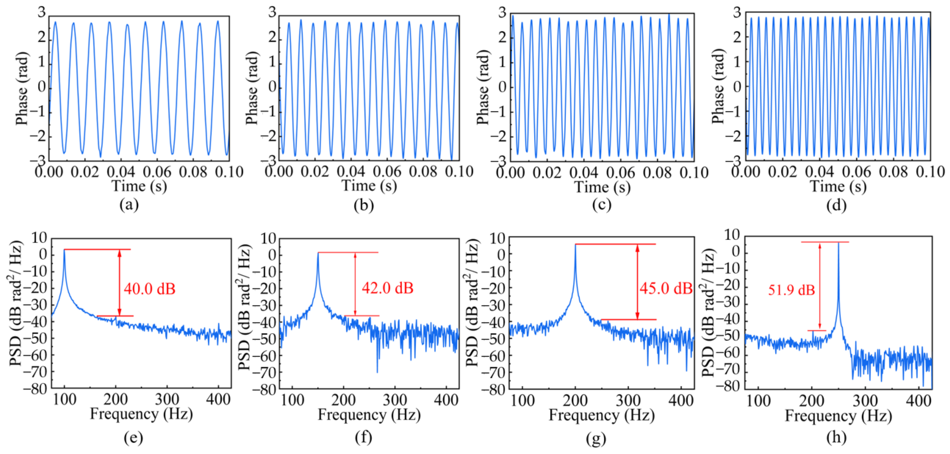
In our study, the accuracy of vibration signal restoration was validated using a Piezoelectric Transducer (PZT) as the vibration source. Multiple sinusoidal signals with peak voltages of 600 mV and frequencies of 100 Hz, 150 Hz, 200 Hz, and 250 Hz were applied to the PZT. By utilizing a φ-OTDR system, the phase evolution chart of the demodulated signal within a time window of 0.1 s was obtained. This approach successfully reconstructed the original vibration signal. The corresponding power spectral density (PSD) is displayed beneath the respective time domain chart in this paper. From Figure 3, it is evident that the peak frequencies in the four sets of PSD charts align precisely with the vibration signal frequencies, thereby confirming the accuracy of vibration signal restoration. The signal-to-noise ratios for the datasets were 40.0 dB, 42.0 dB, 45.0 dB, and 51.9 dB.
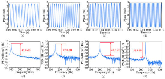
Figure 3.
Phase demodulation results of vibration signals at different frequencies: (a) 100 Hz; (b) 150 Hz; (c) 200 Hz; (d) 250 Hz. Phase demodulation PSD plots of vibration signals at different frequencies: (e) 100 Hz; (f) 150 Hz; (g) 200 Hz; (h) 250 Hz.
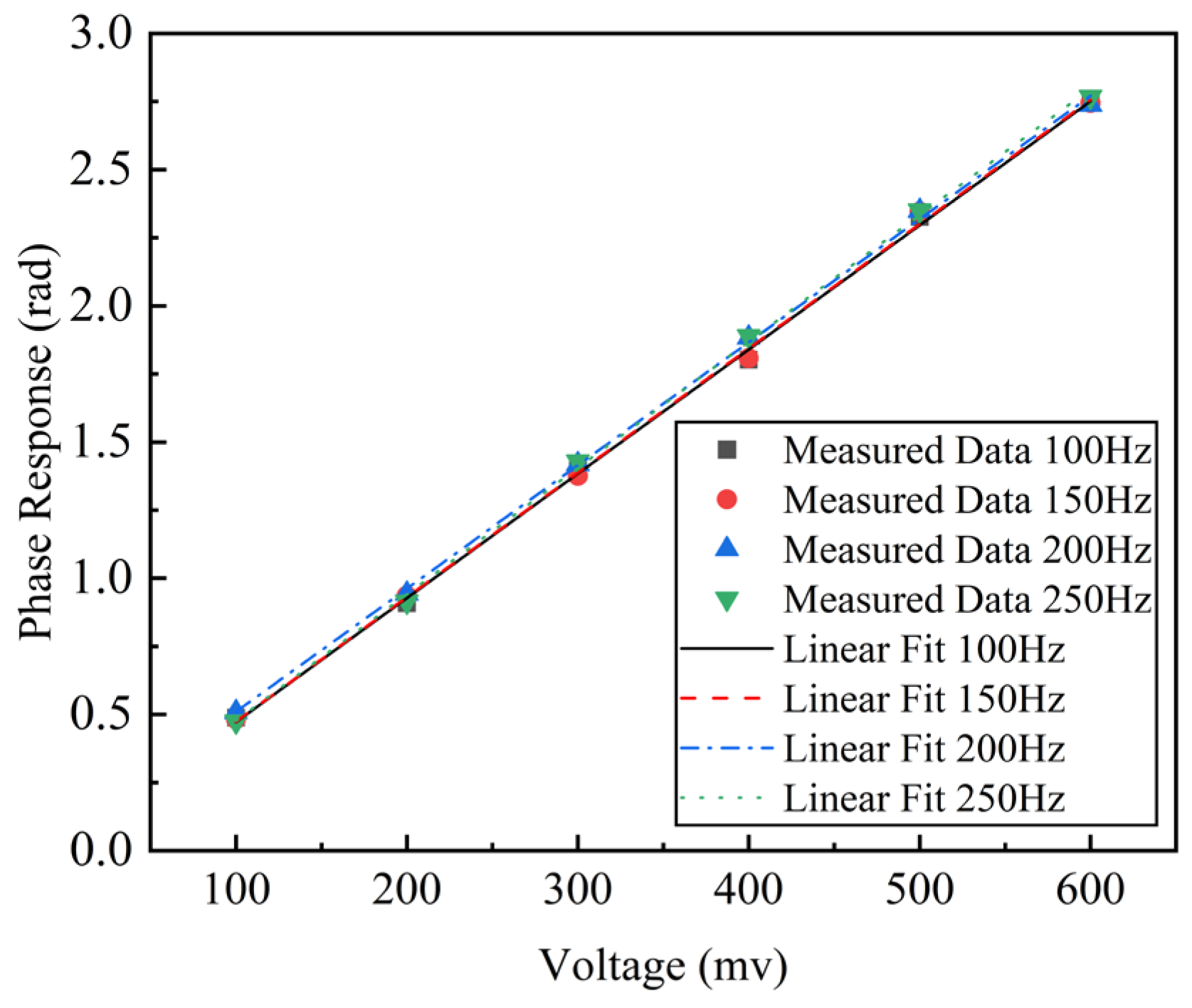
A sinusoidal signal with a frequency of 100 Hz and a peak voltage from 100 mV to 600 mV in 100 mV increments was applied to the PZT, and the corresponding differential phase response peak was recorded. The obtained voltage–phase response curve was linearly fitted to obtain its fitting curve. To demonstrate the reproducibility of the experiment, the above operations were repeated at 150 Hz, 200 Hz, and 250 Hz, and three new fitting curves were obtained; these are summarized and displayed in Figure 4. The slopes of the four curves were almost identical, being 4.56 rad/V, 4.56 rad/V, 4.52 rad/V, and 4.64 rad/V, and the correlation coefficients were 0.99913, 0.99896, 0.99927, and 0.99924, respectively. This confirms the stability and reproducibility of the system’s demodulation.
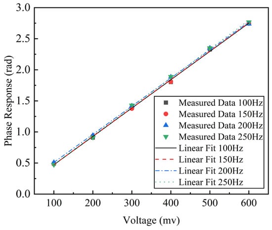
Figure 4.
Phase response results at different voltages and frequencies.
3.3. Dataset Production
The data collection platform in this paper simulates a water pipeline leakage environment. The sensing fiber cable is tightly installed to the water pipeline using nylon ribbon, and an opening is created on the water pipe to simulate a leak. To simulate long-distance detection scenarios, the fiber length is 4 km, and the pulse width is set to 100 ns, corresponding to a spatial resolution of 10 m. Figure 5a is the picture simulating the water pipeline and Figure 5b is the picture of a leakage point, which is a fixed-size hole with a diameter of about 5 mm that is located at the back of the water pipe with a distance of a few centimeters from the sensing cable.
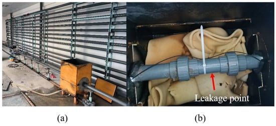
Figure 5.
(a) Simulating water pipeline; (b) leakage point.
Data from operation both with and without leakage events in the water pipe were collected on the aforementioned experimental platform. The data were then divided into training and testing sets. The sample quantities for the two distinct event categories are shown in Table 1, with each individual sample containing 10,240 data points. Figure 6 illustrates five sets of the original phase signals for the water pipe under both non-leakage and leakage conditions. Notably, even during non-leakage periods, the water pipe exhibits low-amplitude, low-frequency vibrations, which are caused by water flow impacting the pipe walls and other environmental disturbances. In addition, since some leakage signals are quite similar to the case of non-leakage, it is difficult to distinguish leakage events through original phase signals.

Table 1.
Number of samples per category.
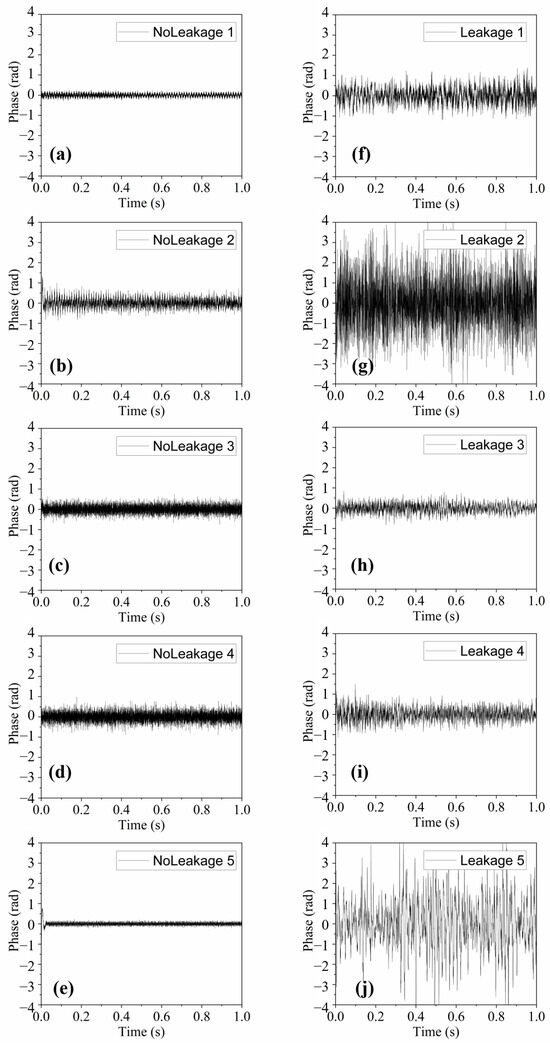
Figure 6.
Phase signals of different events: (a–e) no leakage; (f–j) leakage.
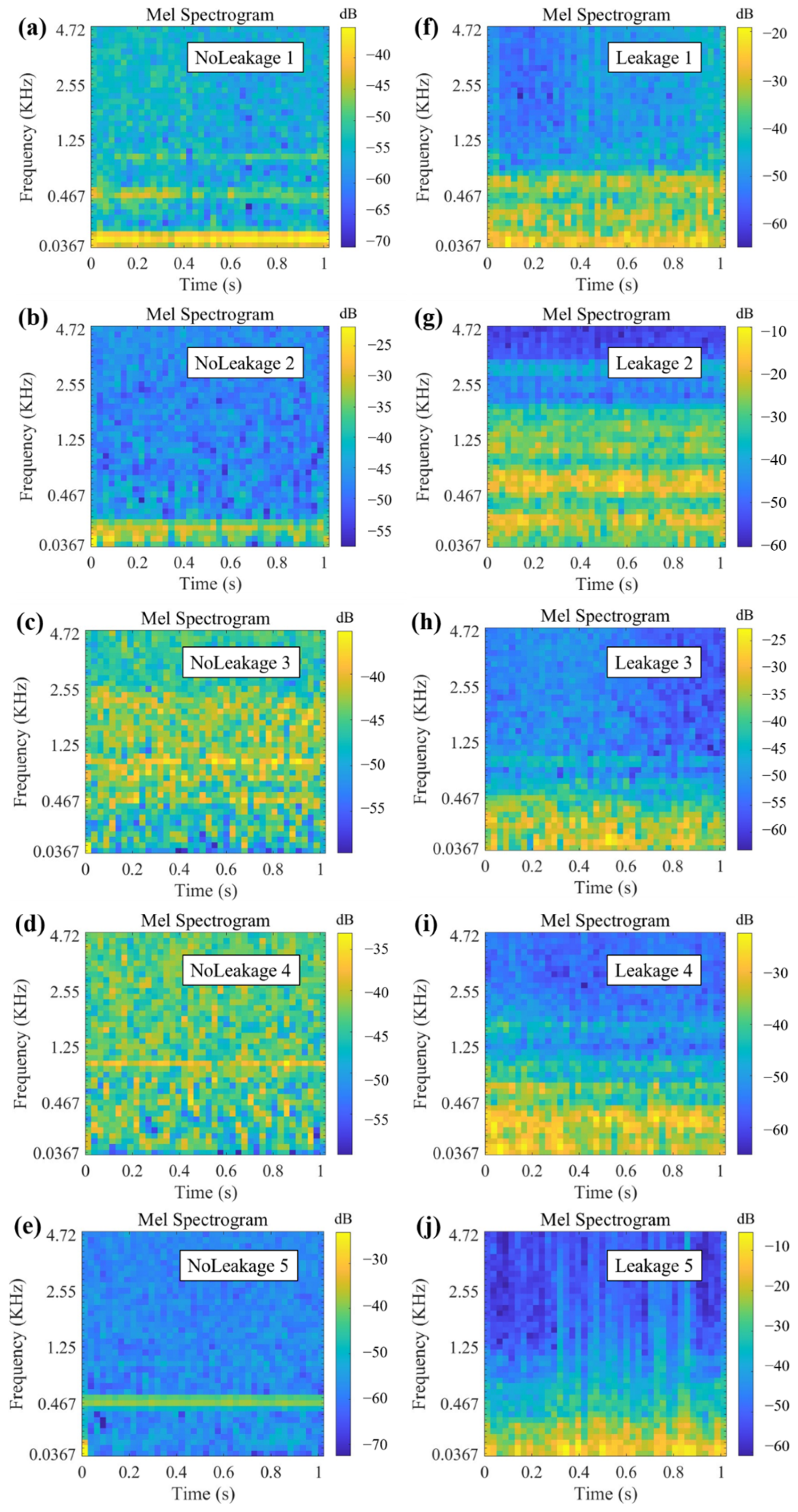
To extract as much effective information as possible from the collected data, original phase data were converted into Mel spectrograms. Mel spectrograms are commonly used in audio signal processing as feature representations. They decompose audio signals into energy distributions across different frequencies, providing richer information. Specifically, Mel spectrograms map linear spectra (typically obtained through Fast Fourier Transform) onto the Mel scale, which better aligns with human auditory perception.
The data were sampled at a rate of 10 KHz, with an FFT window size of 1024 and a frame shift size of 256 and Mel filter number of 40. Figure 7 provides five sets of Mel spectrograms corresponding to both non-leakage and leakage conditions in the water pipe.
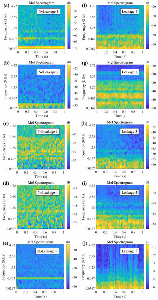
Figure 7.
Mel spectrum diagrams of different events: (a–e) no leakage; (f–j) leakage.
4. Deep Learning Training
4.1. CNN with Mel Spectrograms as Input
When dealing with vibration audio signals, more complex feature representations are often required. Simple one-dimensional data input may not suffice, leading to suboptimal model performance. Therefore, as described in this section, Mel spectrograms were transformed from the one-dimensional phase data, then the Mel spectrograms that served as the input for the CNN model.
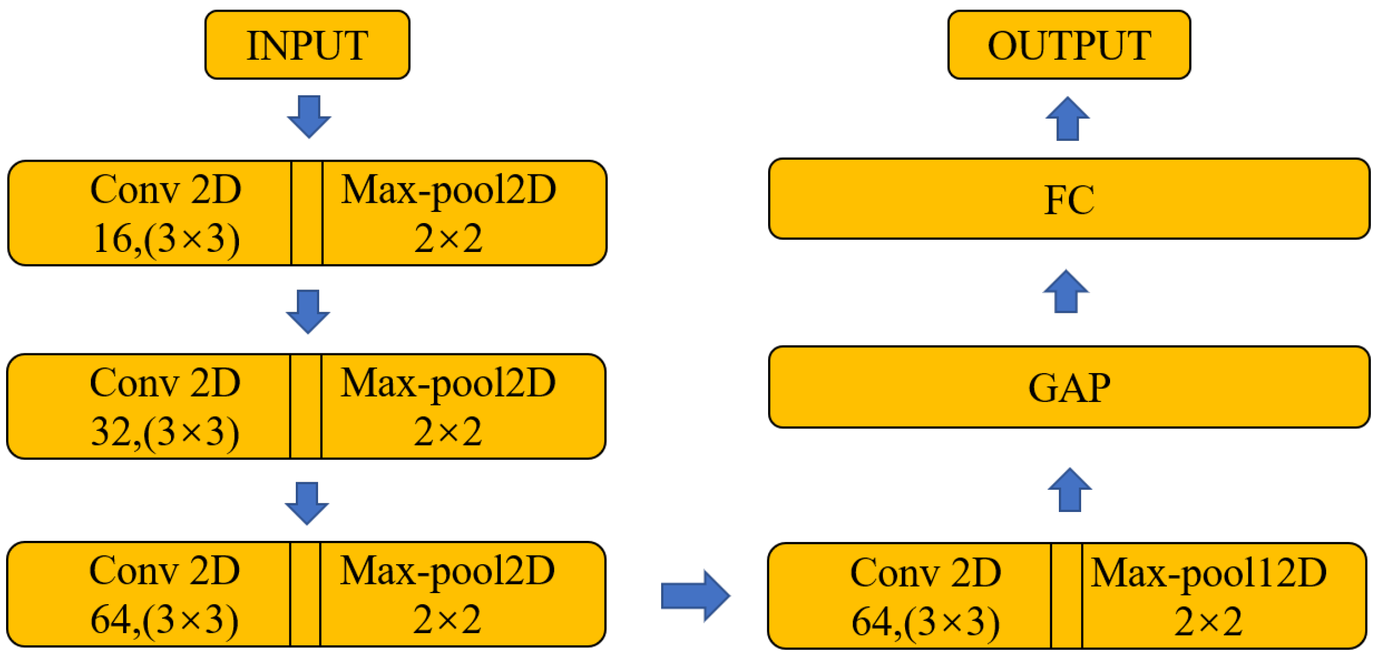
After generating Mel spectrograms, original phase data were transferred into two-dimensional images, where the horizontal axes represented time and the vertical axes represented energy at different frequencies. This allowed us to input them into the CNN model, capturing audio signal features more effectively. The model was built and trained using TensorFlow 2.6 GPU and Python 3.8. When using Mel spectrograms as input data, the corresponding model employs two-dimensional convolutional layers with a kernel size of 3 × 3 and a pooling layer window size of 2 × 2. Other basic settings remain unchanged, and the neural network architecture has been appropriately optimized, as illustrated in the diagram shown in Figure 8:

Figure 8.
Structure of the CNN model. Abbreviations—FC: fully connected layer; GAP: global average pooling.
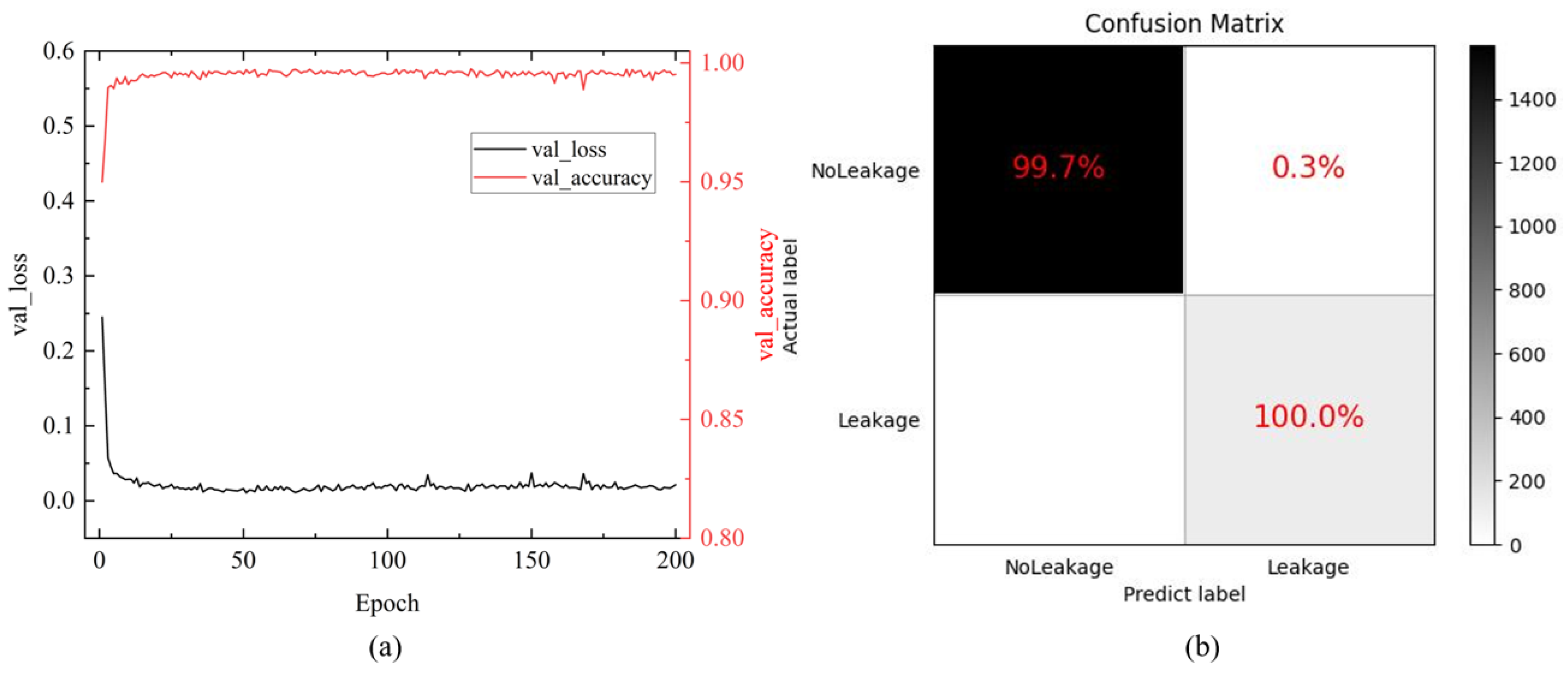
In the process of model training, we continued to utilize the Adam optimizer, with batch size, learning rate, and training epoch values set at 32, 0.001, and 200. The corresponding training curve is depicted in Figure 9a. Using the model, we identified the test dataset and obtained a confusion matrix as shown in Figure 9b. The achieved accuracy was 99.7%.
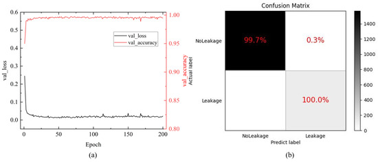
Figure 9.
Training results of the CNN model: (a) training curves; (b) confusion matrix.
4.2. ResNet18 with Mel Spectrograms as Input
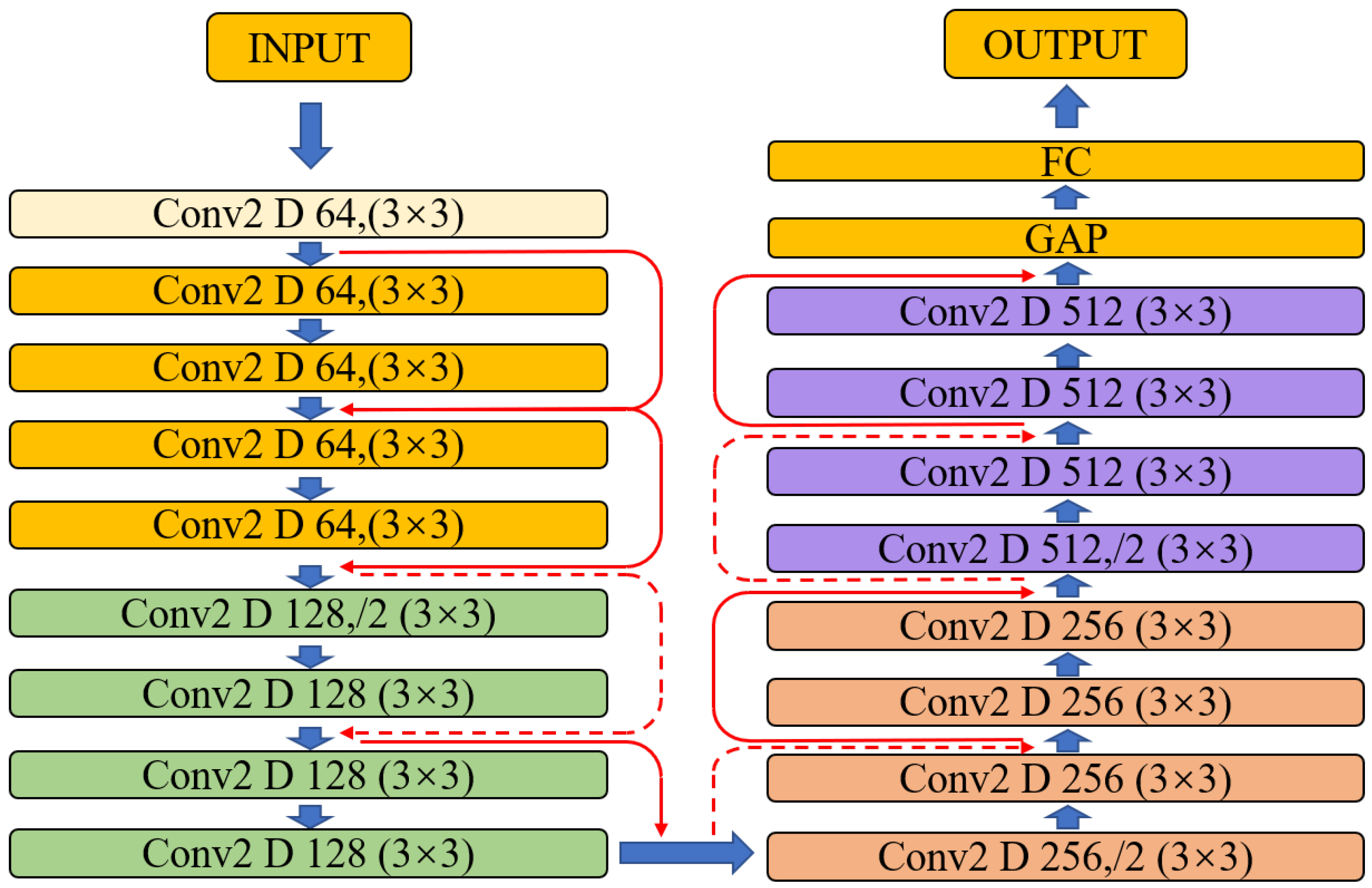
In traditional neural networks, increasing the depth of the network is a common strategy to enhance recognition accuracy by extracting higher-level features from images. However, when the network depth reaches a certain point, the issue of gradient vanishing arises. Deep networks may perform worse than shallow ones due to this phenomenon. To address this challenge, in 2015, He et al. proposed the ResNet18 neural network, which introduced residual blocks with shortcut connections to mitigate gradient vanishing. In conventional deep neural networks, during backpropagation, gradients are multiplied layer by layer with weight matrices, leading to gradual reduction and the eventual disappearance of gradients. In the ResNet model, the shortcut connections directly transmit gradients from the input to subsequent layers, effectively preventing gradient vanishing. A simple residual block structure is illustrated in Figure 10, where input data xi is transformed via weighted operations into f(x) and the final output xi+1 is obtained by adding x and f(x). The specific model architecture is shown in Figure 11.
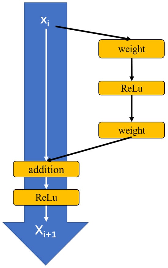
Figure 10.
Residual block structure diagram.
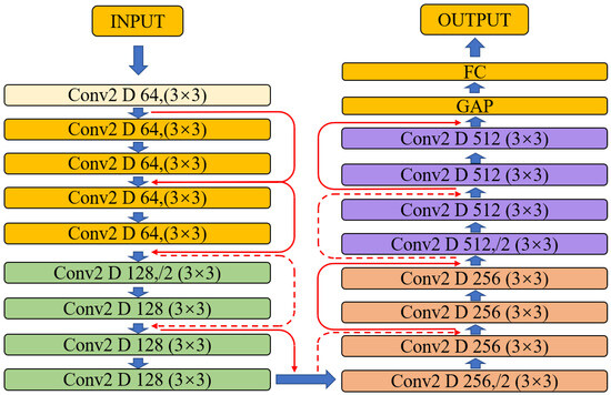
Figure 11.
Structure of the ResNet18 model.
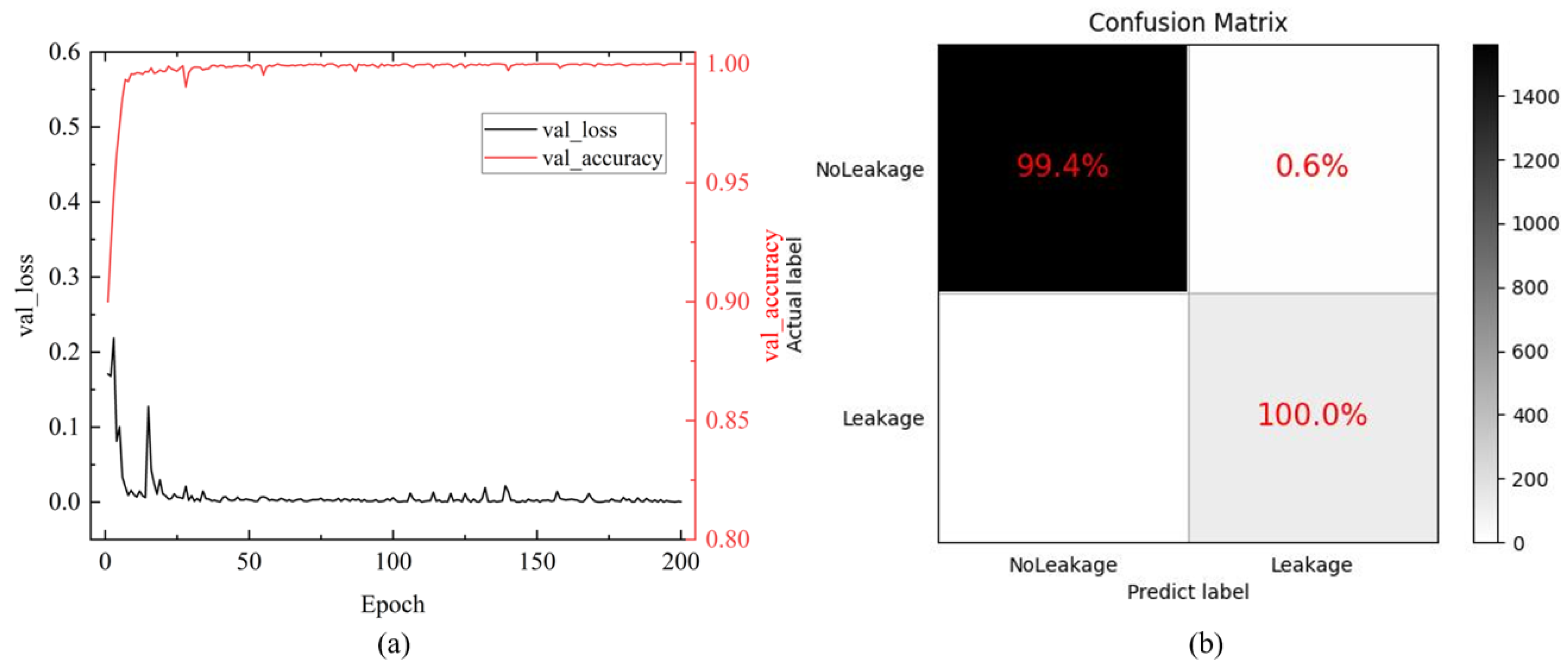
Specifically, ResNet18 consists of multiple residual blocks, each containing two 3 × 3 convolutional layers and a skip connection that adds the original input to the output. These skip connections facilitate the easier training of deep networks. The ResNet18 architecture comprises eighteen layers, including sixteen convolutional layers and two fully connected layers. Convolutional layers are organized into several residual blocks, each incorporating multiple convolutional layers, batch normalization, and ReLU activation. Compared to deeper variants like ResNet50 and ResNet101, ResNet18 strikes a balance between training speed and network depth, with lower complexity and computational resource requirements. In our study, we constructed and trained the ResNet18 model using PyTorch-GPU 0.0.1 and Python 3.8. We adjusted the output dimension of the fully connected layer to 2 for binary classification. Input data consisted of Mel spectrograms derived from raw data. During training, we employed the Adam optimizer with a learning rate of 0.01 and conducted 200 epochs. The corresponding training curve is depicted in Figure 12a. Using the model, we identified the test dataset and obtained a confusion matrix as shown in Figure 12b. The achieved accuracy was 99.5%.
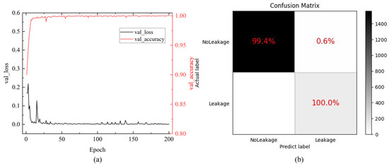
Figure 12.
Training results of the ResNet18 model: (a) training curves; (b) confusion matrix.
4.3. Multi-Leakage Point Detection
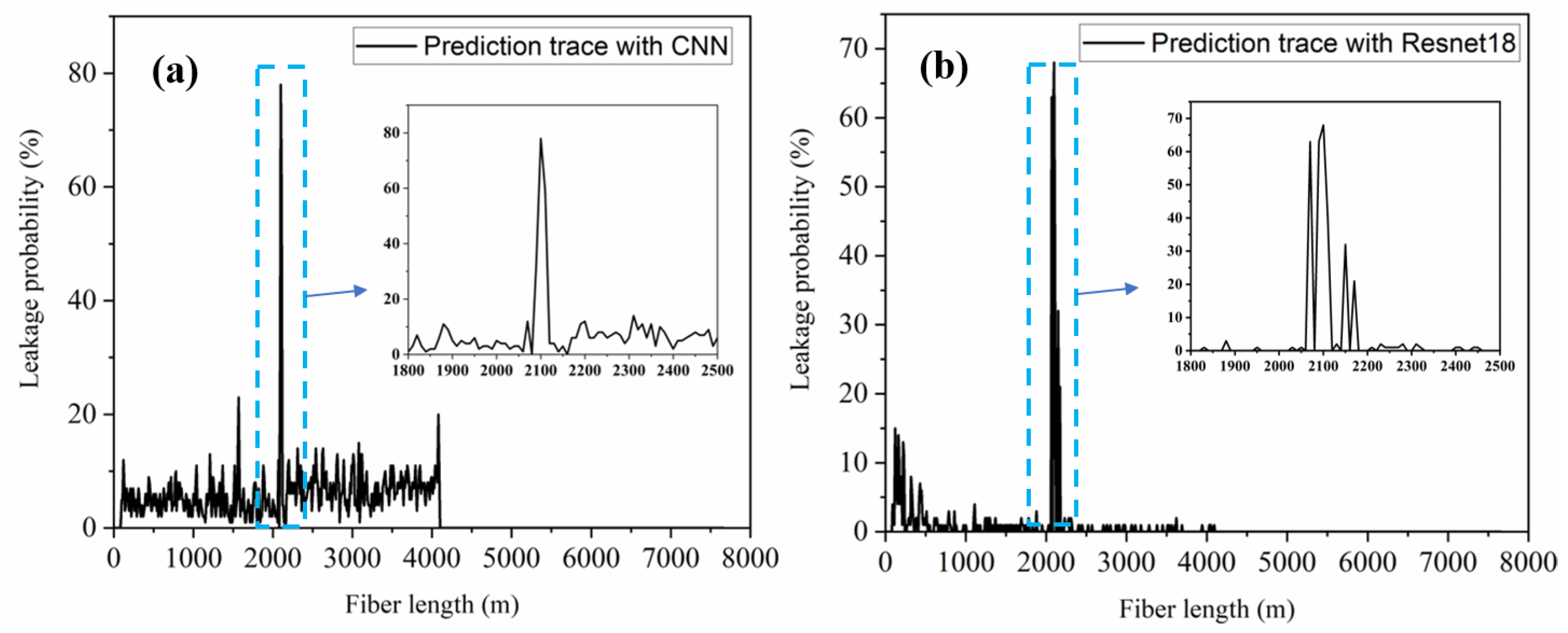
In order to validate and compare the two models described above, we further performed experiments with multiple leak points. In this experiment, three leakage points were set at about 2070 m, 2100 m, and 2150 m from the start of the fiber. The two leak points at 2070 m and 2150 m were simulated by ball valves, and the maximum opening diameter was 20 mm. The leak point at 2100 m was a fixed-size hole with a diameter of about 5 mm. Then, using the phase-sensitive OTDR system described above to collect the experimental data, a total of 100 groups of raw phase data were collected, and each group contained 767 phase data, that is, corresponding to the phase data of all sampling points on the entire FUT. Then, these 100 groups of data were input to the previously trained CNN and ResNet18 models for prediction and to perform statistical analyses of the prediction results, as shown in Figure 13a,b. Experimental results showed that Resnet18 could effectively locate the locations of three leakage points while CNN could only identify leakage events at 2100 m, and the performance of the ResNet18 model at other non-leakage points was also significantly better than that of the CNN model.
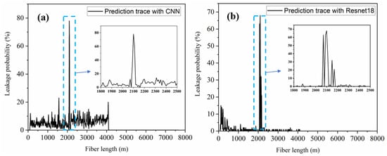
Figure 13.
Multi-leakage points: predicted results of the (a) CNN model and (b) ResNet18 model.
In summary, the CNN and ResNet18 models trained on Mel spectrograms, which contain more informative features, demonstrated good validation accuracy in the classification. However, although, in the previous training and testing phases, the CNN model and the ResNet18 model had similar accuracy, in the multi-leakage point detection experiment, the ResNet18 model performed better, which indicates that Resnet18 has better generalization ability compared to the CNN model when processing new input data. ResNet18 is also the most complex in terms of architecture, computational requirements, and training time.
5. Conclusions
In response to the issue of water pipeline leaks in long-distance transportation, we analyzed, in this paper, the fundamental principles of the phase-sensitive optical time-domain reflectometry system for locating and deciphering disturbance signals. Furthermore, the φ-OTDR system was combined with a deep learning technique to enhance the detection rate of leakage events. By utilizing Mel spectrograms as inputs to a convolutional neural network (CNN) and ResNet18, recognition accuracies of 99.7% and 99.5% were achieved on the validation dataset. In addition, in the multi-leakage point detection experiment, the ResNet18 neural network had better generalization ability compared to the CNN model and successfully located three pre-set leakage points. This has demonstrated that it has good application prospects in the field of monitoring the leakage of long-distance water pipelines.
Author Contributions
Conceptualization, S.W. and S.H.; methodology, S.W. and S.H.; software, S.Z., B.J. and S.W.; validation, S.W. and S.H.; formal analysis, S.Z., Z.Y. and S.W.; investigation, S.Z., Z.X., N.L. and S.W.; resources, S.H.; data curation, S.Z., Z.X. and N.L.; writing—original draft preparation, S.Z.; writing—review and editing, S.W. and S.H.; visualization, S.Z.; supervision, S.W. and S.H.; project administration, S.H.; funding acquisition, S.H. All authors have read and agreed to the published version of the manuscript.
Funding
This work was supported partially by the Ningbo Science and Technology Project (2021Z030, 2023Z179), the National Key Research and Development Program of China (2022YFC3601002), the Key Research and Development Program of Zhejiang Province (2021C03178, 2022C03051, 2023C03135), and the Scientific Research Foundation for Talent Introduction of Zhejiang University’s Ningbo Campus (20201203Z0180).
Institutional Review Board Statement
Not applicable.
Informed Consent Statement
Not applicable.
Data Availability Statement
Data underlying the results presented in this paper are not publicly available at this time but may be obtained from the authors upon reasonable request.
Acknowledgments
The authors are grateful to Julian Evans of Zhejiang University and Wei Chen of Ningbo Water Meter (Group) Company Ltd. for valuable discussions and also grateful to Ningbo Water Meter (Group) Company Ltd. for providing the water leakage test environment.
Conflicts of Interest
The authors declare no conflicts of interest.
References
- Zhuo, L.; Feng, B.; Wu, P. Water Footprint Study Review for Understanding and Resolving Water Issues in China. Water 2020, 12, 2988. [Google Scholar] [CrossRef]
- Momeni, A.; Piratla, K.R. A Proof-of-Concept Study for Hydraulic Model-Based Leakage Detection in Water Pipelines Using Pressure Monitoring Data. Front. Water 2021, 3, 648622. [Google Scholar] [CrossRef]
- Korlapati, N.V.S.; Khan, F.; Noor, Q.; Mirza, S.; Vaddiraju, S. Review and Analysis of Pipeline Leak Detection Methods. J. Pipeline Sci. Eng. 2022, 2, 100074. [Google Scholar] [CrossRef]
- Sousa, D.P.; Du, R.; Mairton Barros da Silva, J., Jr.; Cavalcante, C.C.; Fischione, C. Leakage Detection in Water Distribution Networks Using Machine-Learning Strategies. Water Supply 2023, 23, 1115–1126. [Google Scholar] [CrossRef]
- Peng, L.; Huang, S.; Wang, S.; Zhao, W. A Simplified Lift-Off Correction for Three Components of the Magnetic Flux Leakage Signal for Defect Detection. IEEE Trans. Instrum. Meas. 2021, 70, 6005109. [Google Scholar] [CrossRef]
- Wu, D.; Chatzigeorgiou, D.; Youcef-Toumi, K.; Mekid, S.; Ben-Mansour, R. Channel-Aware Relay Node Placement in Wireless Sensor Networks for Pipeline Inspection. IEEE Trans. Wirel. Commun. 2014, 13, 3510–3523. [Google Scholar] [CrossRef]
- Wu, D.; Chatzigeorgiou, D.; Youcef-Toumi, K.; Ben-Mansour, R. Node Localization in Robotic Sensor Networks for Pipeline Inspection. IEEE Trans. Ind. Inform. 2016, 12, 809–819. [Google Scholar] [CrossRef]
- Mashford, J.; De Silva, D.; Marney, D.; Burn, S. An Approach to Leak Detection in Pipe Networks Using Analysis of Monitored Pressure Values by Support Vector Machine. In Proceedings of the 2009 Third International Conference on Network and System Security, Gold Coast, QLD, Australia, 19–21 October 2009; pp. 534–539. [Google Scholar]
- Leu, S.-S.; Nha, B. Leak Prediction Model for Water Distribution Networks Created Using a Bayesian Network Learning Approach. Water Resour. Manag. 2016, 30, 2719–2733. [Google Scholar] [CrossRef]
- Wu, H.; Sun, Z.; Qian, Y.; Zhang, T.; Rao, Y. A Hydrostatic Leak Test for Water Pipeline by Using Distributed Optical Fiber Vibration Sensing System. In Proceedings of the Fifth Asia-Pacific Optical Sensors Conference, Jeju, Republic of Korea, 20–22 May 2015; Lee, B., Lee, S.-B., Rao, Y., Eds.; SPIE: Bellingham, WA, USA, 2015; p. 965543. [Google Scholar]
- Fu, S.; Zhang, D.; Peng, Y.; Shi, B.; Yedili, N.; Ma, Z. A Simulation of Gas Pipeline Leakage Monitoring Based on Distributed Acoustic Sensing. Meas. Sci. Technol. 2022, 33, 095108. [Google Scholar] [CrossRef]
- Zhu, H.; Pan, C.; Sun, X. Vibration Pattern Recognition and Classification in OTDR Based Distributed Optical-Fiber Vibration Sensing System. Proc. SPIE-Int. Soc. Opt. Eng. 2014, 9062, 906205. [Google Scholar] [CrossRef]
- Jiang, F.; Li, H.; Zhang, Z.; Zhang, Y.; Zhang, X. Localization and Discrimination of the Perturbation Signals in Fiber Distributed Acoustic Sensing Systems Using Spatial Average Kurtosis. Sensors 2018, 18, 2839. [Google Scholar] [CrossRef] [PubMed]
- Samuel, A.L. Some Studies in Machine Learning Using the Game of Checkers. IBM J. Res. Dev. 1959, 3, 210–229. [Google Scholar] [CrossRef]
- Lecun, Y.; Bottou, L.; Bengio, Y.; Haffner, P. Gradient-Based Learning Applied to Document Recognition. Proc. IEEE 1998, 86, 2278–2324. [Google Scholar] [CrossRef]
- He, K.; Zhang, X.; Ren, S.; Sun, J. Deep Residual Learning for Image Recognition. In Proceedings of the 2016 IEEE Conference on Computer Vision and Pattern Recognition (CVPR), Las Vegas, NV, USA, 27–30 June 2016; pp. 770–778. [Google Scholar]
- Jia, H.; Liang, S.; Lou, S.; Sheng, X. A k-Nearest Neighbor Algorithm-Based Near Category Support Vector Machine Method for Event Identification of φ-OTDR. IEEE Sens. J. 2019, 19, 3683–3689. [Google Scholar] [CrossRef]
- Zhang, M.; Li, Y.; Chen, J.; Song, Y.; Zhang, J.; Wang, M. Event Detection Method Comparison for Distributed Acoustic Sensors Using φ-OTDR. Opt. Fiber Technol. 2019, 52, 101980. [Google Scholar] [CrossRef]
- Pan, Z.; Liang, K.; Ye, Q.; Cai, H.; Qu, R.; Fang, Z. Phase-Sensitive OTDR System Based on Digital Coherent Detection. In Proceedings of the 2011 Asia Communications and Photonics Conference and Exhibition (ACP), Shanghai, China, 13–16 November 2011; pp. 1–6. [Google Scholar]
Disclaimer/Publisher’s Note: The statements, opinions and data contained in all publications are solely those of the individual author(s) and contributor(s) and not of MDPI and/or the editor(s). MDPI and/or the editor(s) disclaim responsibility for any injury to people or property resulting from any ideas, methods, instructions or products referred to in the content. |
© 2024 by the authors. Licensee MDPI, Basel, Switzerland. This article is an open access article distributed under the terms and conditions of the Creative Commons Attribution (CC BY) license (https://creativecommons.org/licenses/by/4.0/).

