Abstract
This paper presents the study of decision variables selection in the optimization of sewer network systems. A mathematical model is presented that considers an objective of minimizing the total cost of sewer network comprising all pipe costs, manhole costs, and excavation cost. The mathematical model is solved by using an artificial protozoa optimizer bio-inspired algorithm for the first time in this domain. This work compares ten alternative decision variable sets obtained by systematically varying factors related to the pipe diameter, the slope or cover depths, and nodal elevations. The results display extreme variation among the alternatives. The alternative using only node elevation as a decision variable, that is, Alternative 6, had the lowest average cost, 81345.91, with a very low standard deviation, 28.35, showing maximum consistency. On the other hand, alternatives involving higher numbers of decision variables, such as Alternative 1, resulted in faster computation but with greater variability and cost. Running times ranged from 466 s in Alternative 1 to 66700 s in Alternative 10. The generated alternatives are statistically compared using Friedman and Wilcoxon tests to assess their impact on solution cost and algorithm performance. The results show large variability in the performance consistency and computational efficiency of the alternatives, thus providing indications on the most suitable configurations of decision variables for the sewer network optimization. The alternative which has the nodal elevation as the decision variable performs the best in terms of solution quality. These findings clearly demonstrate that selecting fewer, hydraulically meaningful decision variables can enhance solution quality, although at the expense of increased computational effort.
1. Introduction
Optimization problems consist of objective function(s), decision variables, and constraints. The most important step of optimization is to model the problem mathematically. Determination of decision variables also plays a key role in creating the mathematical model. In some optimization problems, the same problem can be solved with different numbers of decision variables. This situation depends on the decision variables derived from each other. The sewer optimization problem is one of these types of problems. In the literature, sewer system optimization has been traditionally divided into three broad groups: layout optimization, hydraulic optimization, and combined layout and hydraulic optimization. In layout optimization, optimal positions for system elements, such as manholes, pipelines, and pumping stations, are determined to provide efficient flow paths. For instance, Diogo and Graveto [1] made a comparison between deterministic models and stochastic models for layout optimization of sewers. Haghighi [2] introduced a loop-by-loop cut algorithm to develop efficient drainage layouts. Rodrigues et al. [3] created an optimization strategy utilizing a depth-first search to develop optimal layouts for gravity pipe networks. Turan et al. [4] utilized graph theory to develop feasible sanitary sewer networks. A hybrid genetic algorithm has been used by Hassan et al. [5] to develop optimal sewer network layout designs.
Hydraulic optimization is concerned with the best values of the pipe diameters, slopes, and depths, assuming a pre-defined network layout. The earliest cost-based models for branched sewer system optimal design have been proposed by Mays and Yen [6]. Liang et al. [7] presented a hybrid metaheuristic approach by combining genetic algorithms and tabu search to reach more efficient and reliable sewer system hydraulic optimization. Afshar [8] used a genetic algorithm to optimize the storm sewer network, demonstrating the algorithmic usability to treat difficult topologies and constraints. Afshar et al. [9] formulated a hydrograph-based optimization approach using genetic algorithms, which was effective for the simulation of unsteady stormwater flow. Afshar [10] formulated a parameter-free continuous ant colony optimization algorithm for storm sewer systems, both for constrained and unconstrained formulations. Karovic and Mays [11] utilized simulated annealing to solve sewer system optimization problems by using Excel. Duque et al. [12] formulated an optimized procedure for a sewer series of pipes by integrating analytical calculations with hydraulic constraints to reach cost-efficient and technically feasible designs. The usability of genetic algorithms has been improved by Cetin and Yurdusev [13] by adapting the mutation rate dynamically. De Villiers et al. [14] proposed a heuristic algorithm to aid efficient hydraulic optimization for sewer network planning. A two-phase simulation–optimization strategy combining cellular automata with evolutionary algorithms has been proposed by Zaheri et al. [15] for large-scale sewer systems.
A number of studies investigated combined layout optimization and hydraulic optimization. Pan and Kao [16] used a combined GA-QP approach to simultaneously solve layout and hydraulic optimization problems. Navin and Mathur [17] utilized particle swarm optimization (PSO) to optimize both layout and pipe sizes simultaneously. Moeini and Afshar [18] considered an arc-based ant colony optimization method to perform combined gravity-driven network design. Hsie et al. [19] modeled the sewer layout problem as a mixed-integer linear program, inspired by rectilinear Steiner tree algorithms, to reduce the cost of pipes as well as excavation via the utilization of alternative connection nodes. Duque et al. [20] provided an inclusive mathematical framework that combines layout choice with the hydraulic optimization problem with realistic constraints.
Optimization algorithms are used to solve mathematical models after the mathematical model of the problem is obtained. Optimization algorithms are designed to find the best combinations of decision variables’ values for one or more objective functions. These algorithms are utilized in all disciplines, especially economics, basic sciences, or engineering. The effectiveness of optimization algorithms of real-life problems has been proved in many studies [21,22,23,24].
The objective function is considered as the cost of the sewer network; therefore, it consists of the pipe cost, the manhole cost, and the excavation cost. Pipe diameters and pipe slopes that are unknown are sought to minimize the objective function. These unknowns can be directly selected as decision variables, or different variables can be selected as decision variables. In the literature, three different cases are encountered in this matter. In the first case, the pipe diameter, in the second case, the pipe slopes, and in the third case, the pipe diameter and pipe slopes can be selected as decision variables. Constraints consist of lower and upper bounds of velocities and relative flow depths in pipes, lower and upper bounds of slopes, and cover depths. [25]
If the pipe diameter is chosen as the decision variable, the pipe slope and therefore the cover depths can be calculated hydraulically. If the pipe slope or cover depths are chosen as decision variables, the pipe diameter can also be calculated hydraulically. If the pipe diameter and the pipe slope or cover depths are chosen as decision variables, there is no need for hydraulic calculations. So, choosing decision variables also determines the number of decision variables [25].
Different methods such as linear programming, nonlinear programming, and recently meta-heuristic algorithms are used to solve the sewer optimization problem.
When the studies in which different decision variables were made in the sewer optimization problem using meta-heuristic methods are examined, the following studies can be summarized:
Liang et al. [7] used the genetic algorithm and tabu search algorithm in solving the hydraulic optimization problem of the sewer network. Pipe diameter and pipe slope were selected as decision variables. They were applied to the network of The East-I Wastewater Collection Engineering project built in Taiwan.
Afshar et al. [9] used a genetic algorithm in the solution of the hydraulic optimization problem of the sewer network in their study. Two different alternatives were preferred for decision variable selection. In the first alternative, nodal elevation and pipe diameter were selected as decision variables. In the second alternative, only nodal elevation was selected. The application was made on the network proposed by Mays and Wenzel [26].
Izquierdo et al. [27] used the particle swarm algorithm in solving the hydraulic optimization problem of the network in their study. Pipe diameter and pipe slope were selected as decision variables. The application was made on a small network.
Afshar [25] used the rebirthing genetic algorithm in solving the hydraulic optimization problem of the sewer network. A pipe slope was selected as the decision variable. The application was made on the network proposed by Mays and Wenzel [26].
Haghighi and Bakhshipour [28] used an adaptive genetic algorithm in solving the hydraulic optimization problem of the network in their study. Pipe diameter, pipe slope, and pump location were selected as decision variables. The application was made on the network proposed by Li and Matthew [29].
Moeini and Afshar [30] used the ant colony algorithm in their study to solve the hydraulic optimization problem of the sewer network. Nodal elevations were selected as decision variables. The application was made on three different sized networks proposed hypothetically.
Karovic and Mays [11] used the simulated annealing algorithm in their study to solve the hydraulic optimization problem of the network. The upstream crown elevation of the pipe was selected as the decision variable. The application was made on a part of a storm water sewer network.
Navin and Mathur [17] used a particle swarm algorithm in solving the hydraulic optimization problem of the sewer network. Pipe diameter and pipe slope were selected as decision variables. The application was made on the Sudarshanpura, Jaipur, India network.
Tan et al. [31] used the differential evolution algorithm in solving the hydraulic optimization problem of the sewer network in their study. Pipe slope was selected as the decision variable. They applied on the network proposed by Mays and Wenzel [26] and the network of Kerman City, Iran [32].
In the literature, most contributions to sewer network optimization deal either with the development of new solution methods or algorithms’ performance comparison. Apart from these studies, Turan and Çetin [33] presents an alternate viewpoint by investigating the influence of sewer network size on algorithm performance. In the majority of the other hydraulic optimization studies, the choice of decision variables is case-dependent, and the effect of decision variable selection on solution efficiency and computational workload has never been investigated exhaustively employing a fixed network layout and algorithm. Such limitations restrict an in-depth analysis of the influence of decision variable selections on the outcome of optimization and introduce an important gap within the literature that has been under-addressed.
In this study, the effects of decision variable selection on the solution of the sewer hydraulic optimization problem by keeping the network, the method, and parameter values constant have been systematically investigated. With this study, a point that has not been investigated in a controlled manner in literature will be clarified. In addition, the artificial protozoa optimizer (APO) algorithm will be used for the first time in the solution of the sewer optimization problem. For this purpose, solutions were made with ten alternatives where the decision variables were included differently. The results obtained were evaluated statistically with Friedman and Wilcoxon tests in terms of the effect of the decision variable alternatives on the cost and algorithm performance.
2. Methods
2.1. Sewer Network Hydraulic Optimization
The cost of a sewer network consists of the costs of the pipe, manhole, excavation, and pumping station if there is one. The objective function of a sewer network optimization problem without pumping stations can be defined as in Equation (1):
where C is the sewer system cost, N is the total number of sewer pipes, i is the considered pipe, is the unit cost of the sewer pipe construction, is the length of the considered pipe, M is the total number of manholes, j is the considered manhole, and is the cost of the manhole construction. and are defined as a function of the diameter di of the pipe and the manhole height ℎm, respectively. These variables are illustrated in Figure 1.
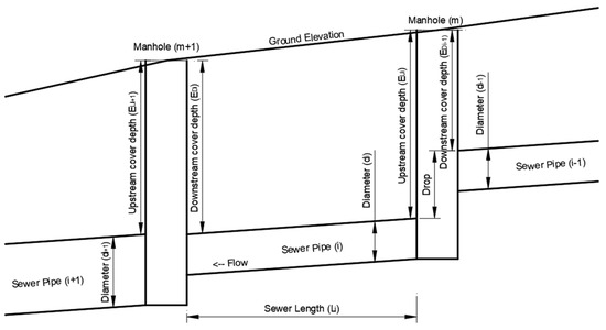
Figure 1.
Schematic representation of the sewer network profile.
The sewer network optimization problem has constraints for hydraulic, operational, and availability reasons. The constraints of this problem can be defined by Equations (2)–(10).
Subject to the following:
where is the diameter of the sewer pipe, is the discrete set of available commercial sewer pipe diameters varying between a minimum diameter value (minD) and maximum diameter value (maxD), is the set of upstream pipe diameters, is the flow velocity of the considered pipe, and are the allowable minimum and maximum velocities, is the relative flow depth value in the considered pipe, and are the allowable minimum and maximum relative flow depth values, is the slope of the considered pipe, is the allowable minimum slope value, is the cover depth value, and and are the allowable minimum (minCD) and maximum (maxCD) cover depth values. In addition to the constraints, in line with the acceptances of the uniform turbulent flow, Manning’s equation is used for hydraulic calculations.
2.2. Artificial Protozoa Optimizer (APO)
The artificial protozoa optimizer (APO) is a recent bio-inspired metaheuristic algorithm proposed with the goal of dealing with complex optimization problems for different applications, ranging from engineering design to image segmentation [34]. APO derives inspiration from protozoa’s survival mechanisms, more particularly considering foraging, dormancy, and reproductive behavior. In return, these behaviors contribute to the algorithm’s capacity of exploring and exploiting search space. In this section, a detailed account of the algorithm, along with its mathematical models and pseudo code for implementation, is presented.
The algorithm starts by initializing the initial solutions and parameters of the algorithm, such as the population size and the maximum number of function evaluations. This lets the algorithm get into the state before the iterative process of optimization starts. The optimization loop begins by checking if the termination criteria; in this case, the maximum number of evaluations (MaxFEs) is met. If the condition is satisfied, the algorithm stops; otherwise, it proceeds to the next step. At this level, the population’s protozoa are ranked according to their fitness values. The ranking made here is important because it is what permits the algorithm to classify the protozoa in terms of the performance regarding the optimization problem. Following the classification, the algorithm performs an evaluation of the behavior exhibited by each of the protozoa and determines the course of foraging, dormancy, or reproduction. This is the most critical process in the decision mechanism, and the adaptability and efficiency of the APO algorithm strongly rely on it. For protozoa during the foraging process, the algorithm differentiates autotrophic and non-autotrophic ones. Autotrophic protozoa generate new protozoa with a particular foraging behavior modeled by Equation (11). The general equation of foraging behavior modeled by Equation (12) is used to express the foraging behavior of non-autotrophic protozoa. Protozoa in the dormancy state give rise to new protozoa following the behavior depicted by Equation (13). Dormancy behavior is modeled to represent how the protozoa can survive in unfavorable situations through reduced activity and energy preservation. On the other hand, protozoa not in the dormancy state reproduce to produce new protozoa following Equation (14). Reproduction is carried out as a process whereby the population is diversified and continuously improved from new genetic materials. After the foraging, dormancy, or reproduction, the algorithm updates the evaluation and updating of the protozoa population. The newly generated protozoa are then evaluated for their fitness, and the population is updated with those individuals. If a better solution to this evaluation is found, the global optimum solution is also updated.
The steps of the optimization loop are carried out until some predefined termination criteria are met. Through this iterative population improvement and utilization of the different behaviors of protozoa, the APO algorithm becomes competent to navigate its solution space towards finding an optimal solution. When the maximum allowable number of function evaluations is conducted or another stopping condition satisfied, the algorithm stops and gives the best solution found so far. This detailed approach makes the APO algorithm remain robust, adaptive, and efficient in solving complex optimization problems.
Here, represents the new position of the protozoan, and is its current time step position. denotes a randomly picked up the position of some other protozoan, and np is the total number of pairs for neighboring. The autotrophic mode weight factor helps in updating the movement of the protozoan as a function of the neighbors’ positions, such as and . The factor f represents the foraging factor, which decides upon the step size, and indicates mapping vector to decide which dimension of the protozoan position needs to be modified.
In this equation, is a position of a nearby nutrient-rich region and is the weight factor in heterotrophic mode. The protozoan locates towards for exploiting nutrient sources with f controlling the magnitude of the move while gives the updated dimensions.
Here, and represent the lower and upper bounds of the search space, respectively, while is a random vector with elements in the range [0, 1].
In this equation, is the current position of the protozoan, and represents the new position after reproduction. The scalar introduces randomness, and is the mapping vector for reproduction.
Few critical parameters form the basis upon which the artificial protozoa optimizer algorithm can regulate the optimization process so as to ensure effectiveness: the number of protozoa, a candidate solution from the population of size specified by ps, such that the larger the value, the more the number of protozoa, the greater the diversity, at the cost of computational cost; dim specifies the dimensionality within the optimization problem, i.e., the number of decision variables, structuring the search space that protozoa will traverse. The number of neighbor pairs (np) is considered during a foraging to align the positions of protozoans based on the influences from neighbors, thus helping in exploration and exploitation. MaxFEs bound the algorithm, defining the stopping criterion. Proportion fraction of dormancy and reproduction (pf) and its upper limit (pfmax) control the balance between introducing new solutions and exploiting those of high quality. An important factor, the foraging factor (f), controls the adaptive step size of the foraging process to balance exploration and exploitation. In this formulation, the autotrophic () and heterotrophic () weight factors modulate the dynamics of the movement towards the light source and nutrient-rich areas, respectively. Lastly, an adaptive setting of the probability of autotrophic and heterotrophic behavior (pah) determines the propensity to exhibit either foraging mode, gradually shifting the movement from a state of exploration to one of exploitation over iterations. The trade-off between entering the dormancy stage and reproduction is controlled by the pdr. The parameter values of the APO algorithm were chosen based on the recommendations of the initial study by Wang et al. [34].
The flowchart of the APO algorithm is given in Figure 2.
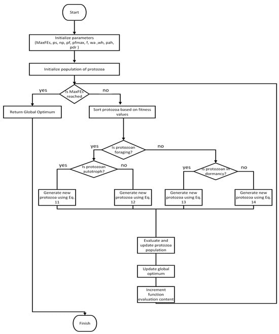
Figure 2.
Flowchart of APO algorithm.
2.3. Selection of Decision Variables
Decision variables are variables that correspond to the minimum or maximum value of the objective function according to the problem and whose values are aimed at being determined by solving the optimization problem. It is stated that the objective function of the sewer network hydraulic optimization problem consists of the pipe cost, manhole cost, and excavation cost. The pipe cost is calculated depending on the pipe length, pipe material, and pipe diameter. For a network with a pre-defined layout and pipe type, the pipe cost will vary only depending on the pipe diameter, since the pipe lengths and pipe type are fixed. The manhole cost is calculated depending on the number of manholes, type of the manhole, and manhole depths. For a sewer network with a pre-defined layout and manhole type, the manhole cost will vary only depending on the manhole depth since the number of manholes and the manhole type are fixed. Finally, excavation cost is calculated depending on the excavation volume, the soil structure, and the excavation technique. For a sewer network with a uniform soil structure, pre-defined layout, excavation width, and excavation technique, the excavation cost will vary only depending on the excavation depth. In this specific problem, these variables can be directly selected as decision variables, or these variables can be indirectly calculated with each other to create different decision variable sets. In literature, three different cases are encountered in this sense. In the first case, the pipe diameter, in the second case, the pipe slopes, and in the third case, the pipe diameter and pipe slopes can be selected together as decision variables. If the pipe diameter is selected as the decision variable, the pipe slope, and therefore the excavation depths, can be determined by hydraulic calculations. If the decision variable is selected as the slope or depths, the pipe diameter can be obtained by hydraulic calculations. If the pipe diameter and the slope or depths are selected as the decision variables, there is no need for hydraulic calculations.
In this context, 10 different alternative sets of decision variables are created in this study. The alternative sets are obtained by allowing or not allowing drops in the network, using cover depths, the nodal elevation values or slope values, and the diameter. A summary of information about alternative sets is given in Table 1.

Table 1.
Alternative set of decision variables.
As seen from Table 1, a different number of decision variables are utilized in different decision variable alternative sets. In Alternative 1, 2, 4, 7, and 9, drops in manholes are allowed, while in other alternatives, drops in manholes are not allowed.
2.4. Constraint Handling
The inverse tangent method is used as the constraint handling method in this study. In this method, the maximum value of constraint violations () is taken as the fitness value. On the other hand, if the constraints are not violated, the arc tangent of the objective value is taken as fitness value. The process is given in Equation (15).
where represents the arc tangent function [35].
3. Application
In this study, the network of Kerman City, which was proposed by Mansouri and Khanjani [32], is used. The layout and the characteristics of this network are given in Figure 3 and Table 2, respectively. There are 21 manholes and 20 lines in the network. Design parameters of this network, summarized in Table 3, such as minimum and maximum velocity values, minimum and maximum relative flow depth, minimum cover depth value, and manning coefficient and diameter sets, are taken from Hassan, etc. [36].
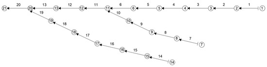
Figure 3.
The layout of the Kerman network [32].
Table 2.
Characteristics of the network.
Table 3.
Design parameters of the network.
In this study, the total cost function of the network is used as Equation (18), which was proposed by Mansouri and Khanjani [32]:
where is the cost of pipe installations, is the considered pipe, is the diameter of the considered pipe, is the average excavation depth of the considered pipe, is the cost of manhole installations, and is the height of the manhole.
As stated by Hassan et al. [36], some researchers studying on the same network used 2.45 m as the minimum cover depth value, while others used this same value as the minimum depth of excavation known as the minimum invert. This inconsistency leads to differences in cost estimates from one study to another. In this study, 2.45 m is taken as the minimum cover depth value.
Some assumptions must be made to solve the problem. Furthermore, the search space reduction is utilized to improve computational efficiency by limiting the solution space. Details of this process are given below.
In Alternatives 1, 2, 3, 5, 9, and 10, for inlets of the network, the lower and upper bounds of the diameter values are minD and maxD. For downstream lines at the manhole in these alternative sets, the lower and upper bounds of the diameter value are the maximum diameter value of upstream lines connected to the same manhole and maxD. In Alternatives 4, 6, 7, and 8, the diameter of the line satisfying hydraulic constraints is searched from minD to maxD for inlets and from the maximum diameter values of incoming lines to maxD for the lines other than the inlets.
In Alternatives 1, 4, 5, and 6, for the inlets of the network, the lower and upper bounds of the upstream cover depth values are minCD and maxCD. On the other hand, in Alternatives 2, 3, 7, 8, 9, and 10 that are decision variable sets not including cover depth values, there must be a cover depth value assumption for selected manholes of the network. For this reason, the upstream cover depth values of all inlets in Alternatives 2, 7, and 9 that are drop-allowed sets, and the inlets in Alternatives 3, 8, and 10 that are not drop-allowed sets, are assigned as minCD.
In Alternatives 1 and 4 for all downstream lines, the lower and upper bounds of upstream cover depth value are the maximum downstream cover depth value of upstream lines connected to the same manhole and maxCD. In Alternatives 2, 3, 5, 6, 7, 8, 9, and 10 for all downstream lines, the upstream cover depth values of downstream lines are assigned as the maximum downstream cover depth values of upstream lines connected to the same manhole.
In Alternatives 9 and 10, the slope of each line is searched for the minimum value that satisfies hydraulic constraints.
In Alternatives 3, 8, and 10, since there is no drop in the manhole where there is more than one connection from upstream lines and to downstream lines, all cover depth values of manholes are assigned as the same value if there is one cover depth value calculated before.
In Alternatives 1, 2, 4, 5, 6, 7, and 9, the calculation process starts from one of the inlets and proceeds through the outlet. On the other hand, in Alternatives 3, 8, and 10, the calculation process begins at one of the inlets and continues until the intersection manhole. At the intersection manhole, the calculation process proceeds from the intersection manhole to the other inlet. After reaching the second inlet, calculation resumes from the intersection manhole to the outlet.
The APO parameters, i.e., the population size and the maximum number of iterations, are determined as 50 and 10000, respectively. Moreover, to evaluate the results statistically, each trial was run 30 times.
4. Results and Discussions
Table 4 summarizes the computational results of the 10 alternatives, 1 to 10 with the number of decision variables (# DV): minimum (Min), maximum (Max), average (Avg), standard deviation (Std), and average computational times in seconds (Time) over a total of 30 runs.
Table 4.
Computational results.
Figure 4 depicts the four principal measures of performance minimum cost, average cost, standard deviation, and average computation time for all alternatives normalized to their corresponding maximum values. The figure makes it easier to perform a complete, multi-dimensional analysis of each decision variable configuration’s overall profile of performance.
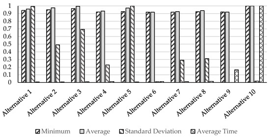
Figure 4.
Normalized computational results.
Meanwhile, Alternatives 6 and 9 have much more predictable behavior. That means that their results are mostly the same in every execution. These alternatives might be preferred in scenarios where consistency and reliability come first. While Alternatives 1, 3, and 5 show the highest variability in performance, Alternatives 6 and 9 are the most consistent. Whichever decision criterion is used, whether it is average performance or consistency, different alternatives would be preferred to solve the problem at hand.
The table of average computational times provides valuable insights into the efficiency of each Alternatives 1 to 10. The results show a wide range of computational times, with the fastest alternative being Alternative 1. Alternatives 1, 2, and 5 may be preferable in time-sensitive applications where quick results are critical. In contrast, Alternatives such as 9 and 10 stand out for their extremely high computational times. These alternatives would be less desirable in scenarios where time efficiency is crucial, even if Alternative 9 provides good performance metrics in terms of objective function values.
From Table 4, it is observed that the alternatives with fewer decision variables have longer average computational times. In this respect, the average computational times of Alternatives 1, 2, 3, and 5 are below the rest. The alternatives where diameter and slope values are not decision variables take significantly longer in computational time. It should be noted that, for example, Alternatives 9 and 10, which have neither slope nor cover depth as decision variables, are significantly longer compared with Alternative 1, which computes the shortest time. In alternatives which have the same decision variables and have different drop characteristics, namely, 2-3, 7-8, and 9-10, alternatives with drop allowed tend to be longer in average computational times.
Alternatives 6, 7, 8, 9, and 10, which have the fewest decision variables, perform lower minimum and average cost values that indicate better performance. Likewise, these alternatives also have lower standard deviation, which shows more consistent results. In alternatives which have the same decision variables and have different drop characteristics, namely, 2-3, 7-8, and 9-10, alternatives with drop allowed tend to be lower results.
There seems to be a performance versus CPU time trade-off. Alternative spars in terms of decision variables, such as 5 and 6, presented good objective values but take longer to compute, while more dense alternatives, such as 1 and 2, solved faster but presented greater variability and less optimal performance. Herein, this may refer to the fact that a reduced number of decision variables could improve the solution quality, albeit at the price of longer computation times.
Alternative 10 seems to be an outlier. With 20 decision variables, it has one of the highest averages, 6670.82, and its minimum and maximum, also average, are not that good. Hence, sometimes even fewer decision variables do not guarantee either good performance or faster computation in certain cases. It could be due to the fact that there is some other kind of complexity in the problem which does not relate to the number of decision variables.
While generally better performance may be achieved with fewer decision variables, the average computation times are longer. Perhaps more decision variables reduce computational time but yield solutions that are less optimal and have higher variability. The choice of alternatives depends on whether the priority is faster computation or higher-quality performance.
The alternatives are also compared through non-parametric statistical tests, namely the Friedman test and Wilcoxon signed-rank test. The statistical results are given in Table 5.
Table 5.
Statistical test results.
The Friedman test is used to rank the alternatives based on their performance across multiple runs. The alternatives are ranked from 1 (best) to 10 (worst), with the sum of ranks indicating the overall performance of each alternative. Alternative 6 emerges as the top-performing alternative, with the lowest sum of ranks (1.07). This suggests that Alternative 6 consistently performed better than the other alternatives in most of the test cases.
The Wilcoxon signed-rank test examines the statistical significance of the differences in performance between Alternative 6 and the other alternatives. For the alternatives 1, 2, 3, 4, 5, 8, 9, and 10, the p-value is extremely small (approximately 1.73 × 10−06). This indicates that Alternative 6 significantly outperforms these alternatives, and its performance is significantly better than the other alternatives statistically as p < 0.01. For Alternative 7, the p-value is slightly higher but still very small (5.75 × 10−06), indicating that while Alternative 6 is better, the performance difference is still statistically significant. The low p-values confirm that Alternative 6 is consistently superior to the other alternatives in terms of performance.
Alternative 6 is clearly the top-performing alternative based on both the Friedman ranking and the Wilcoxon signed-rank test. It outperforms all other alternatives with a high level of statistical significance.
The statistical significance indicated by the Wilcoxon signed-rank test highlights that the differences between Alternative 6 and other alternatives are not due to random variation, further validating Alternative 6 as the most reliable option for the problem at hand.
Alternative 6 has a total of 21 decision variables. All these decision variables are nodal elevation. In this case, after determining the nodal elevations, other values are obtained by hydraulic calculations.
5. Conclusions
This research thoroughly evaluated for the first time in the literature under fully controlled settings the effects of selection of decision variables on the solution quality of the sewer network hydraulic optimization problem. For this, the network topology, parameter settings, and optimization algorithms were maintained at a constant. At the stage of solving, the artificial protozoa optimizer algorithm was chosen as a neutral and unbiased schema, and it was implemented for the first time within this research area.
Ten different alternatives for decision variables were considered within the research. Alternative 6, using nodal elevations as decision variables, resulted in the minimum average cost (81345.91) as well as the maximum consistency (standard deviation: 28.35). Alternative 6 ranked highest by the results of the Friedman test and proved to be superior to all other alternatives at a statistical significance of p less than 0.01 by the Wilcoxon signed-rank test.
On the other hand, Alternatives 1 and 5 took shorter computation times (466.39 and 483.92 s) but at a greater cost and variability. Alternatives 9 and 10 were extremely consistent, with a near-zero standard deviation, but were at a disadvantage because of using extremely long computation times (10987.28 and 66700.82 s) and having greater total costs (81488.87 and 88623.63).
It is evident from these findings that selection of decision variables is crucial to obtaining optimum solutions for sewer system planning that are both efficient and cost-effective.
Numerous research efforts in the literature revolved around innovative solution methodologies or the comparison of different approaches’ efficiency for sewer network optimization. In contrast to these efforts, the innovation of the present work is based on a systematic comparison of the impacts of various decision variable settings on optimization solutions under the same circumstances. To a certain extent, this research bridges a major knowledge gap for the literature and provides grounds for innovation in potential future research efforts.
In subsequent research, the use of environmental and economic sustainability as decision variable dimensions and parallel computing approaches might reduce computation times while increasing the realism of the optimization process.
Author Contributions
Conceptualization, T.C., M.E.T. and M.E.S.; methodology, T.C., M.E.T. and M.E.S.; software, T.C., M.E.T. and M.E.S.; validation, T.C., M.E.T. and M.E.S.; formal analysis, T.C., M.E.T. and M.E.S.; data curation, T.C. and M.E.T.; writing—original draft preparation, T.C., M.E.T. and M.E.S.; writing—review and editing, T.C., M.E.T. and M.E.S.; visualization, T.C., M.E.T. and M.E.S. All authors have read and agreed to the published version of the manuscript.
Funding
This research was funded by Manisa Celal Bayar University Scientific Research Projects Coordination Unit. Project Number: 2024-047.
Institutional Review Board Statement
Not applicable.
Informed Consent Statement
Not applicable.
Data Availability Statement
The original contributions presented in the study are included in the article, further inquiries can be directed to the corresponding author.
Conflicts of Interest
The authors declare no conflicts of interest.
References
- Diogo, A.F.; Graveto, V.M. Optimal Layout of Sewer Systems: A Deterministic Versus a Stochastic Model. J. Hydraul. Eng. 2006, 132, 927–943. [Google Scholar] [CrossRef]
- Haghighi, A. Loop-by-Loop Cutting Algorithm to Generate Layouts for Urban Drainage Systems. J. Water Resour. Plan. Manag. 2013, 139, 693–703. [Google Scholar] [CrossRef]
- Rodrigues, G.P.W.; Costa, L.H.M.; Farias, G.M.; Castro, M.A.H. A Depth-First Search Algorithm for Optimizing the Gravity Pipe Networks Layout. Water Resour. Manag. 2019, 33, 4583–4598. [Google Scholar] [CrossRef]
- Turan, M.E.; Bacak-Turan, G.; Cetin, T.; Aslan, E. Feasible Sanitary Sewer Network Generation Using Graph Theory. Adv. Civ. Eng. 2019, 2019, 8527180. [Google Scholar] [CrossRef]
- Hassan, W.H.; Attea, Z.H.; Mohammed, S.S. Optimum Layout Design of Sewer Networks by Hybrid Genetic Algorithm. J. Appl. Water Eng. Res. 2020, 8, 108–124. [Google Scholar] [CrossRef]
- Mays, L.W.; Yen, B.C. Optimal Cost Design of Branched Sewer Systems. Water Resour. Res. 1975, 12, 37–47. [Google Scholar] [CrossRef]
- Liang, L.Y.; Thompson, R.G.; Young, D.M. Optimising the Design of Sewer Networks Using Genetic Algorithms and Tabu Search. Eng. Constr. Archit. Manag. 2004, 11, 101–112. [Google Scholar] [CrossRef]
- Afshar, M.H. Application of a Genetic Algorithm to Storm Sewer Network Optimization. Sci. Iran. 2006, 13, 234–244. [Google Scholar]
- Afshar, M.H.; Afshar, A.; Mariño, M.A.; Darbandi, A.A.S. Hydrograph-Based Storm Sewer Design Optimization by Genetic Algorithm. Can. J. Civ. Eng. 2006, 33, 319–325. [Google Scholar] [CrossRef]
- Afshar, M.H. A Parameter Free Continuous Ant Colony Optimization Algorithm for the Optimal Design of Storm Sewer Networks: Constrained and Unconstrained Approach. Adv. Eng. Softw. 2010, 41, 188–195. [Google Scholar] [CrossRef]
- Karovic, O.; Mays, L.W. Sewer System Design Using Simulated Annealing in Excel. Water Resour. Manag. 2014, 28, 4551–4565. [Google Scholar] [CrossRef]
- Duque, N.; Duque, D.; Saldarriaga, J.A. New Methodology for the Optimal Design of Series of Pipes in Sewer Systems. J. Hydroinformatics 2016, 18, 757–772. [Google Scholar] [CrossRef]
- Cetin, T.; Yurdusev, M.A. Genetic Algorithm for Networks with Dynamic Mutation Rate. Gradevinar 2017, 69, 1101–1109. [Google Scholar] [CrossRef]
- De Villiers, N.; Van Rooyen, G.C.; Middendorf, M. Sewer Network Design: Heuristic Algorithm for Hydraulic Optimisation. J. S. Afr. Inst. Civ. Eng. 2017, 59, 48–56. [Google Scholar] [CrossRef][Green Version]
- Zaheri, M.M.; Ghanbari, R.; Afshar, M.H. A Two-Phase Simulation–Optimization Cellular Automata Method for Sewer Network Design Optimization. Eng. Optim. 2020, 52, 620–636. [Google Scholar] [CrossRef]
- Pan, T.-C.; Kao, J.-J. GA-QP Model to Optimize Sewer System Design. J. Environ. Eng. 2009, 135, 17–24. [Google Scholar] [CrossRef]
- Navin, P.K.; Mathur, Y.P. Design Optimization of Sewer System Using Particle Swarm Optimization. In Advances in Intelligent Systems and Computing, Proceedings of Fifth International Conference on Soft Computing for Problem Solving; Pant, M., Deep, K., Bansal, J., Nagar, A., Das, K., Eds.; Springer: Singapore, 2016; Volume 437. [Google Scholar] [CrossRef]
- Moeini, R.; Afshar, M.H. Arc Based Ant Colony Optimization Algorithm for Optimal Design of Gravitational Sewer Networks. Ain Shams Eng. J. 2017, 8, 207–223. [Google Scholar] [CrossRef]
- Hsie, M.; Wu, M.-Y.; Huang, C.Y. Optimal Urban Sewer Layout Design Using Steiner Tree Problems. Eng. Optim. 2019, 51, 1980–1996. [Google Scholar] [CrossRef]
- Duque, N.; Duque, D.; Aguilar, A.; Saldarriaga, J. Sewer Network Layout Selection and Hydraulic Design Using a Mathematical Optimization Framework. Water 2020, 12, 3337. [Google Scholar] [CrossRef]
- Preitl, Z.; Precup, R.E.; Tar, J.K.; Takács, M. Use of Multi-Parametric Quadratic Programming in Fuzzy Control Systems. Acta Polytech. Hung. 2006, 3, 29–43. [Google Scholar]
- Paliszkiewicz, J. Knowledge Management: An Integrative View and Empirical Examination. Cybern. Syst. 2007, 38, 825–836. [Google Scholar] [CrossRef]
- Zapata, H.; Perozo, N.; Angulo, W.; Contreras, J. A Hybrid Swarm Algorithm for Collective Construction of 3D Structures. Int. J. Artif. Intell. 2020, 18, 1–18. [Google Scholar]
- Precup, R.-E.; David, R.-C.; Roman, R.-C.; Petriu, E.M.; Szedlak-Stinean, A.-I. Slime Mould Algorithm-Based Tuning of Cost-Effective Fuzzy Controllers for Servo Systems. Int. J. Comput. Intell. Syst. 2021, 14, 1042–1052. [Google Scholar] [CrossRef]
- Afshar, M.H. Rebirthing Genetic Algorithm for Storm Sewer Network Design. Sci. Iran. 2012, 19, 11–19. [Google Scholar] [CrossRef]
- Mays, L.W.; Wenzel, H.G. Optimal Design of Multilevel Branching Sewer Systems. Water Resour. Res. 1976, 12, 913–917. [Google Scholar] [CrossRef]
- Izquierdo, J.; Montalvo, I.; Pérez, R.; Fuertes, V.S. Design Optimization of Wastewater Collection Networks by PSO. Comput. Math. Appl. 2008, 56, 777–784. [Google Scholar] [CrossRef]
- Haghighi, A.; Bakhshipour, A.E. Optimization of Sewer Networks Using an Adaptive Genetic Algorithm. Water Resour. Manag. 2012, 26, 3441–3456. [Google Scholar] [CrossRef]
- Li, G.; Matthew, R.G.S. New Approach for Optimization of Urban Drainage Systems. J. Environ. Eng. 1990, 116, 927–944. [Google Scholar] [CrossRef]
- Moeini, R.; Afshar, M.H. Constrained Ant Colony Optimisation Algorithm for the Layout and Size Optimisation of Sanitary Sewer Networks. Urban Water J. 2013, 10, 154–173. [Google Scholar] [CrossRef]
- Tan, E.; Sadak, D.; Ayvaz, M.T. Kanalizasyon Sistemlerinin Diferansiyel Evrim Algoritması Kullanılarak Optimum Tasarımı. Teknik Dergi 2020, 31, 10229–10250. [Google Scholar] [CrossRef]
- Mansouri, M.R.; Khanjani, M.J. Optimization of Sewer System by the Nonlinear Programming. J. Water Wastewater 1999, 10, 20–30. (In Persian) [Google Scholar]
- Turan, M.E.; Cetin, T. Analyzing the Effect of Sewer Network Size on Optimization Algorithms’ Performance in Sewer System Optimization. Water 2024, 16, 859. [Google Scholar] [CrossRef]
- Wang, X.; Snášel, V.; Mirjalili, S.; Pan, J.-S.; Kong, L.; Hisham, A.S. Artificial Protozoa Optimizer (APO): A Novel Bio-Inspired Metaheuristic Algorithm for Engineering Optimization. Knowl.-Based Syst. 2024, 295, 111737. [Google Scholar] [CrossRef]
- Kim, H.; Maruta, I.; Sugie, T. A Simple and Efficient Constrained Particle Swarm Optimization and Its Application to Engineering Design Problems. Proc. Inst. Mech. Eng. C J. Mech. Eng. Sci. 2010, 224, 389–400. [Google Scholar] [CrossRef]
- Hassan, W.H.; Jassem, M.H.; Mohammed, S.S. A GA-HP Model for the Optimal Design of Sewer Networks. Water Resour. Manag. 2018, 32, 865–879. [Google Scholar] [CrossRef]


Disclaimer/Publisher’s Note: The statements, opinions and data contained in all publications are solely those of the individual author(s) and contributor(s) and not of MDPI and/or the editor(s). MDPI and/or the editor(s) disclaim responsibility for any injury to people or property resulting from any ideas, methods, instructions or products referred to in the content. |
© 2025 by the authors. Licensee MDPI, Basel, Switzerland. This article is an open access article distributed under the terms and conditions of the Creative Commons Attribution (CC BY) license (https://creativecommons.org/licenses/by/4.0/).